MutSeqR: Analyzing Mutation Frequencies

Load MutSeqR and Example Data

library(MutSeqR)

library(ExperimentHub)
# load the index
eh <- ExperimentHub()

Generalized Linear Modeling

An important component of analysing mutagencity data is how mutation frequency (MF) changes based on experimental variables.

The model_mf() function can be used to quantitatively evaluate how MF changes based on experimental variables. The function models the proportion of reads that carry a mutation (i.e. the MF) across user-supplied fixed and/or random effects and interaction parameters. Depending on the supplied effects, model_mf() will automatically choose to fit either a generalized linear model (GLM) using the glm() function from the stats library or a generalized linear mixed model (GLMM) using the glmer() function from the lme4 library.

Model Formula

Fixed effects: The experimental variable(s)/factor(s) of interest.
Random effects: Variable used to account for variability within a larger group. Covariate.
Interaction: The product of two or more interacting fixed_effects. An interaction implies that the effect of one fixed effect changes depending on the levels of another fixed effect, indicating a non-additive reationship.
Response: the function will model the MF, taking the mutation count (sum) and the group_depth as input.

The model formula is built as:

cbind(sum, group_depth) ~ fixed_effect1 + fixed_effect2 + ... + (1|random_effect)

If test_interaction is set to TRUE, the model will use the product of the fixed_effects:

cbind(sum, group_depth) ~ fixed_effect1 * fixed_effect2 * ... + (1|random_effect)

Family

The occurence of mutations is assumed to follow a binomial distribution as:

There is a finite number of sequenced bases.
A mutation at any given base is equally probable*.
Mutations occur independently of other mutations.

We acknowledge that this does not reflect biological reality.

To account for over-dispersion, the function will fit a GLM with a quasibinomial distribution. If the dispersion parameter of the model is less than 1, the model will be refit using a binomial distribution. The GLMM will always use a binomial distribution.

The model_mf function will fit a generalized linear model to analyse the effect(s) of given fixed_effects(s) on MF and perform specified pairwise comparisons between levels of your factors.

Additional arguments can be passed to the model to further customize it to your needs. Details on the arguments for the generalized linear model can be found at stats::glm and for the general linear mixed model at lme4::glmer.

Estimates & Comparisons

model_mf() provides estimates of the mean for each level of the fixed effects. Furthermore, pairwise comparisons can be performed based on a user-supplied table. Mean estimates and comparisons are conducted using the doBy R library (doBy?). Estimates of the back-transformed standard errors are approximated using the delta method. The p-values are adjusted for multiple comparisons using the Sidak method.

Goodness of Fit

The model_mf function will output the Pearson residuals appended to the mf_data. The row with the highest residual will be printed to the console so that users may assess it as an outlier. Additionally, Pearson residuals will be plotted as a histogram and a QQ-plot to check for deviances from model assumptions. We assume that residuals will follow a normal distribution with a mean of 0. Thus, we expect the histogram to follow a bell curve and the QQ-plot to be plotted along the y=x line.

General Usage

Mutation data should first be summarised by sample using calculate_mf(). The mf_data should be output as a summary table. Be sure to retain the columns for experimental variables of interest using the retain_metadata_cols parameter.

You may specify factors and covariates for your model using the fixed_effects and random_effects parameters respectively. If more than one fixed_effect is supplied, then you may specify whether you wish to test the interaction between your fixed_effects using the test_interaction parameter. For each fixed effect, you must also include the reference level using the reference_level parameter. The level specified as the reference level will be used as the intercept when calculating model coefficients.

You must specify the columns in your mf_data that contain the mutation counts and the total_depth per sample using the muts and total_counts parameters respectively. Default values should be sufficient if the mf_data was created using calculate_mf().

To perform pairwise comparisons between levels of your fixed effects, supply a constrast table using the contrasts parameter. This can either be a data frame or a filepath to a text file that will be loaded into R. The table must consist of two columns, each containing levels within the fixed_effects. The level in the first column will be compared to the level in the second column for each row.

If the user supplies multiple fixed effects to the model, then each value in the contrasts table must include levels for all fixed_effects. Within each value, the levels of the different fixed_effects should be seperated by a colon. For example, if we have fixed effects dose and tissue, one comparison might be control:lung vs. control:heart. The function will calculate the fold-difference in MF of the first column relative to the second column. The function will also provide the p-value denoting the significance of the difference. If you specify multiple pairwise comparisons, then the p-values will automatically be corrected for multiple comparisons using the Sidak method.

Output

The function will output a list of results.

model: the glmm or glmer model object.
model_formula: the formula given to glm or glmer.
model_data: the supplied mf_data with added column for Pearson residuals.
summary: the summary of the model.
anova: the analysis of variance for models with two or more fixed_effects. See car::Anova..
residuals_histogram: the Pearson residuals plotted as a histogram. This is used to check whether the variance is normally distributed. A symmetric bell-shaped histogram, evenly distributed around zero indicates that the normality assumption is likely to be true.
residuals_qq_plot: the Pearson residuals plotted in a quantile-quantile plot. For a normal distribution, we expect points to roughly follow the y=x line.
point_estimates_matrix: the contrast matrix used to generate point-estimates for the fixed effects.
point_estimates: the point estimates for the fixed effects.
pairwise_comparisons_matrix: the contrast matrix used to conduct the pairwise comparisons specified in the contrasts.
pairwise_comparisons: the results of pairwise comparisons specified in the contrasts.

Examples

Example 1. Model by Dose

Example 1. Model the effect of dose on MF. Our example data consists of 24 mouse samples, exposed to 3 doses of BaP or a vehicle control. Dose Groups are : Control, Low, Medium, and High. We will determine if the MFmin of each BaP dose group is significantly increased from that of the Control group. Example data is the same as that used in the vignette. See the vignette for information on importing and filtering the data.

First, we will calculate MF per sample while retaining the dose column.

# load example data:
example_data <- eh[["EH9861"]]

mf_data_global <- calculate_mf(
  mutation_data = example_data,
  cols_to_group = "sample",
  subtype_resolution = "none",
  retain_metadata_cols = c("dose_group", "dose")
)

Next, we will build a contrasts table that compares each BaP dose group back to the control group.

# Create a contrasts table for pairwise comparisons
contrasts_table <- data.frame(
  col1 = c("Low", "Medium", "High"),
  col2 = c("Control", "Control", "Control")
)

Finally, we will run the model.

# Run the model
model_by_dose <- model_mf(
  mf_data = mf_data_global,
  fixed_effects = "dose_group",
  muts = "sum_min",
  total_count = "group_depth",
  reference_level = "Control",
  contrasts = contrasts_table
)

Residuals Histogram

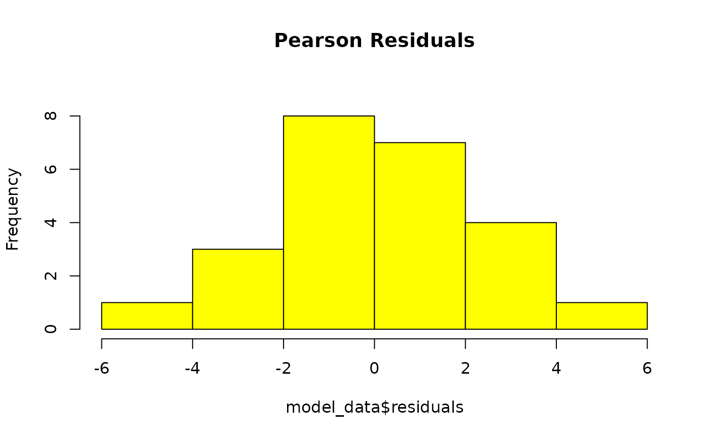
GLM residuals of MFmin modelled as an effect of Dose. x is pearson’s residuals, y is frequency. Plotted to validate model assumptions. n = 24.

The residuals form a bell-curve with a mean of 0 indicating that they follow a normal distribution.

Residuals QQ-plot

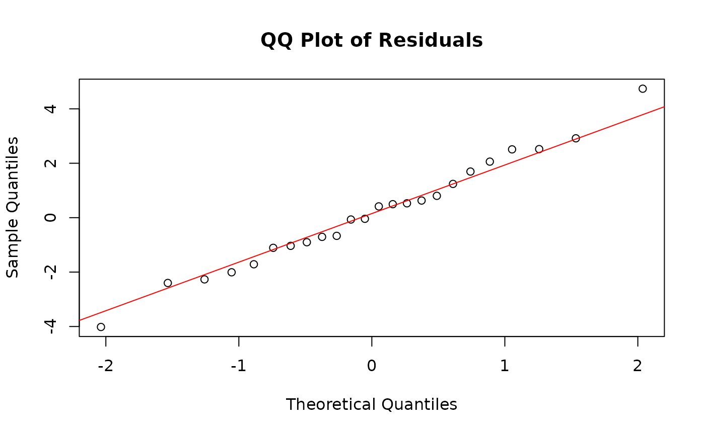
GLM residuals of MFmin modelled as an effect of Dose expressed as a quantile-quantile plot. Y is the pearson’s residuals of the model in ascending order x is the quantiles of standard normal distribution for n of 24. Plotted to validate model assumptions.

The QQ-plot depicts points ollowing the y=x line, indicating that residuals follow a normal distribution. Our model assumptions have been validated.

Model Summary

model_by_dose$summary

## 
## Call:
## stats::glm(formula = model_formula, family = "quasibinomial", 
##     data = mf_data)
## 
## Coefficients:
##                   Estimate Std. Error  t value Pr(>|t|)    
## (Intercept)      -15.56285    0.08290 -187.736  < 2e-16 ***
## dose_groupHigh     1.69485    0.08915   19.011 2.84e-14 ***
## dose_groupLow      0.67512    0.10066    6.707 1.58e-06 ***
## dose_groupMedium   1.29746    0.09563   13.567 1.51e-11 ***
## ---
## Signif. codes:  0 '***' 0.001 '**' 0.01 '*' 0.05 '.' 0.1 ' ' 1
## 
## (Dispersion parameter for quasibinomial family taken to be 4.604243)
## 
##     Null deviance: 2919.634  on 23  degrees of freedom
## Residual deviance:   89.569  on 20  degrees of freedom
## AIC: NA
## 
## Number of Fisher Scoring iterations: 5

The model summary indicates that dose group has a significant effect on mutation frequency. Our model fit a quasibiniomal model with a low dispersion parameter (4.6) indicating a good fit.

Model Estimates

Table 18. model_by_dose$point_estimates: Estimated Mean Mutation Frequency per Dose.

The point estimates returns the mean values estimated by the model for each level of the fixed effects. We can compare these values to the empirical mean that is calculated directly from our data to check that the model fit the data well.

Pairwise Comparisons

Table 19. model_by_dose$pairwise_comparisons

We performed pairwise comparisons to determine which dose groups were significantly different from control. The pairwise comparisons were performed based on the contrasts table supplied to model_mf(). Our results show that the mutation frequency is signifincatly increased for all dose groups relative to the control group, ranging from a 2-fold increase in the Low dose group to a 5.5-fold increase in the High dose group.

Due to the novelty of using ECS for mutagenicity assessmnent, there are no widely established thresholds for what constitutes a biologically meaningful change. However, previous guidelines for interpreting biological relevance, derived from traditional mutagenicity assays, recommend a minimum fold change of 1.5 (White et al., 2020).

Example 2. Model by Dose and Target

Example 2. Model the effects of dose and genomic locus on MF. Sequencing for the example data was done on a panel of 20 genomic targets. We will determine if the MF of each BaP dose group is significantly different from the Control individually for all 20 targets. In this model, dose group and target label will be our fixed effects. We include the interaction between the two fixed effects. Because sample will be a repeated measure, we will use it as a random effect. See the vignette for more information on how we imported and filtered this dataset.

First, calculate MF for each sample and genomic locus, while retaining the dose column.

mf_data_rg <- calculate_mf(
  mutation_data = example_data,
  cols_to_group = c("sample", "label"),
  subtype_resolution = "none",
  retain_metadata_cols = "dose_group"
)

Next, create a contrasts table the compares each dose group back to the control for each genomic locus:.

combinations <- expand.grid(dose_group = unique(mf_data_rg$dose_group),
                            label = unique(mf_data_rg$label))
combinations <- combinations[combinations$dose_group != "Control", ]
combinations$col1 <- with(combinations, paste(dose_group, label, sep = ":"))
combinations$col2 <- with(combinations, paste("Control", label, sep = ":"))
contrasts2 <- combinations[, c("col1", "col2")]

Finally, run the model. As this model is more complex, we will improve covergence by supplying the control argument, which is passed directly to lme4::glmer().

model_by_target <- model_mf(mf_data = mf_data_rg,
  fixed_effects = c("dose_group", "label"),
  test_interaction = TRUE,
  random_effects = "sample",
  muts = "sum_min",
  total_count = "group_depth",
  contrasts = contrasts2,
  reference_level = c("Control", "chr1"),
  control = lme4::glmerControl(optimizer = "bobyqa",
                               optCtrl = list(maxfun = 2e5))
)

Residuals Histogram

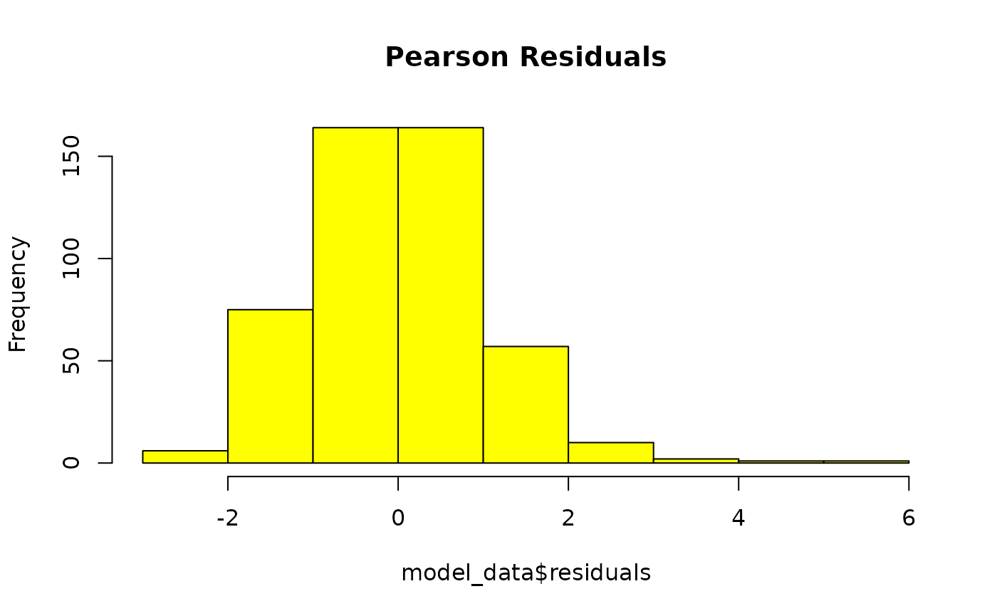
GLMM residuals of MFmin modelled as an effect of Dose and Genomic Target. x is pearson’s residuals, y is frequency. Plotted to validate model assumptions. n = 24.

Residuals QQ-plot

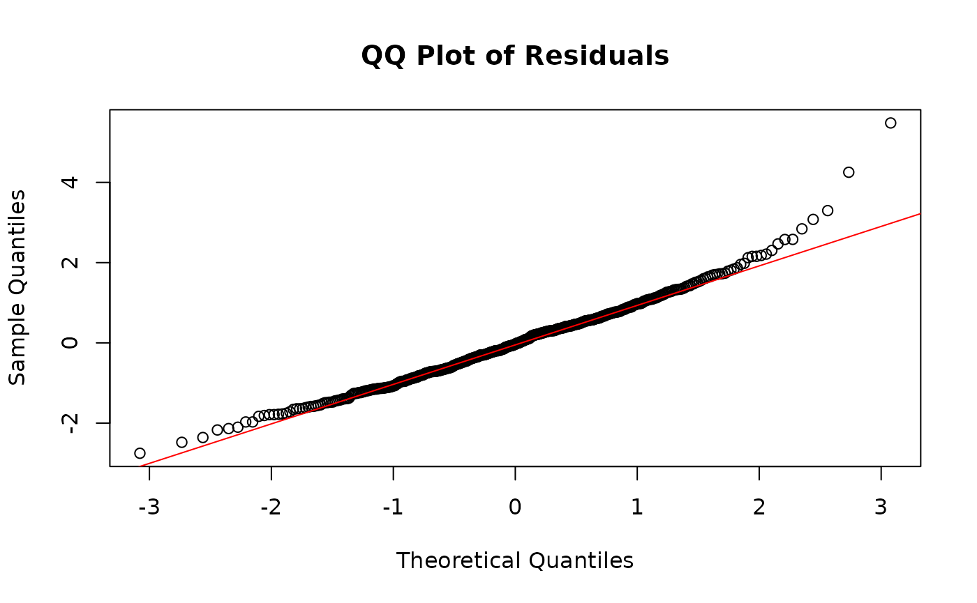
GLMM residuals of MFmin modelled as an effect of Dose and Genomic Target expressed as a quantile-quantile plot. Y is the pearson’s residuals of the model in ascending order x is the quantiles of standard normal distribution for n of 24. Plotted to validate model assumptions.

The histogram and the QQ plot indicate normally distributed residuals.

Model Summary

model_by_target$summary

## Generalized linear mixed model fit by maximum likelihood (Laplace
##   Approximation) [glmerMod]
##  Family: binomial  ( logit )
## Formula: cbind(sum_min, group_depth) ~ dose_group * label + (1 | sample)
##    Data: mf_data
## Control: ..1
## 
##       AIC       BIC    logLik -2*log(L)  df.resid 
##    2825.5    3163.6   -1331.7    2663.5       399 
## 
## Scaled residuals: 
##     Min      1Q  Median      3Q     Max 
## -2.7513 -0.7140 -0.0326  0.6138  5.4812 
## 
## Random effects:
##  Groups Name        Variance Std.Dev.
##  sample (Intercept) 0.01088  0.1043  
## Number of obs: 480, groups:  sample, 24
## 
## Fixed effects:
##                                Estimate Std. Error z value Pr(>|z|)    
## (Intercept)                  -1.596e+01  2.222e-01 -71.807  < 2e-16 ***
## dose_groupHigh                1.903e+00  2.395e-01   7.947 1.92e-15 ***
## dose_groupLow                 6.208e-01  2.738e-01   2.267 0.023380 *  
## dose_groupMedium              1.293e+00  2.612e-01   4.951 7.39e-07 ***
## labelchr1.2                   1.382e-01  2.824e-01   0.489 0.624624    
## labelchr10                    4.517e-01  2.682e-01   1.684 0.092109 .  
## labelchr11                    8.366e-01  2.641e-01   3.168 0.001535 ** 
## labelchr12                    5.183e-01  2.660e-01   1.948 0.051365 .  
## labelchr13                    1.984e-02  2.908e-01   0.068 0.945593    
## labelchr14                    6.560e-01  2.671e-01   2.456 0.014043 *  
## labelchr15                    5.084e-01  2.660e-01   1.911 0.056012 .  
## labelchr16                    7.757e-01  2.693e-01   2.881 0.003970 ** 
## labelchr17                    4.593e-01  2.885e-01   1.592 0.111307    
## labelchr18                   -7.519e-03  2.958e-01  -0.025 0.979721    
## labelchr19                   -2.378e-01  3.084e-01  -0.771 0.440585    
## labelchr2                     6.258e-01  2.660e-01   2.352 0.018661 *  
## labelchr3                     2.568e-01  2.863e-01   0.897 0.369732    
## labelchr4                     5.106e-01  2.773e-01   1.841 0.065603 .  
## labelchr5                     4.209e-01  2.824e-01   1.490 0.136186    
## labelchr6                     2.937e-01  2.806e-01   1.046 0.295350    
## labelchr7                    -3.983e-04  2.958e-01  -0.001 0.998926    
## labelchr8                     4.383e-01  2.908e-01   1.507 0.131704    
## labelchr9                     7.000e-01  2.671e-01   2.621 0.008766 ** 
## dose_groupHigh:labelchr1.2   -2.483e-01  3.022e-01  -0.822 0.411347    
## dose_groupLow:labelchr1.2    -2.540e-03  3.459e-01  -0.007 0.994141    
## dose_groupMedium:labelchr1.2 -2.494e-02  3.289e-01  -0.076 0.939548    
## dose_groupHigh:labelchr10    -4.750e-01  2.882e-01  -1.648 0.099285 .  
## dose_groupLow:labelchr10     -3.356e-01  3.360e-01  -0.999 0.317857    
## dose_groupMedium:labelchr10  -3.318e-01  3.167e-01  -1.048 0.294861    
## dose_groupHigh:labelchr11    -5.554e-02  2.809e-01  -0.198 0.843268    
## dose_groupLow:labelchr11      4.252e-01  3.174e-01   1.340 0.180390    
## dose_groupMedium:labelchr11   4.359e-01  3.029e-01   1.439 0.150068    
## dose_groupHigh:labelchr12    -1.676e-01  2.836e-01  -0.591 0.554373    
## dose_groupLow:labelchr12     -1.544e-01  3.287e-01  -0.470 0.638477    
## dose_groupMedium:labelchr12  -1.756e-01  3.115e-01  -0.564 0.572958    
## dose_groupHigh:labelchr13    -3.978e-01  3.125e-01  -1.273 0.202970    
## dose_groupLow:labelchr13      2.170e-03  3.561e-01   0.006 0.995138    
## dose_groupMedium:labelchr13  -2.386e-01  3.425e-01  -0.697 0.486037    
## dose_groupHigh:labelchr14     1.207e-01  2.832e-01   0.426 0.670094    
## dose_groupLow:labelchr14      2.822e-01  3.228e-01   0.874 0.381936    
## dose_groupMedium:labelchr14   4.877e-01  3.055e-01   1.596 0.110378    
## dose_groupHigh:labelchr15    -1.145e+00  2.935e-01  -3.903 9.51e-05 ***
## dose_groupLow:labelchr15     -4.122e-01  3.348e-01  -1.231 0.218290    
## dose_groupMedium:labelchr15  -6.712e-01  3.214e-01  -2.088 0.036792 *  
## dose_groupHigh:labelchr16    -2.607e-01  2.878e-01  -0.906 0.364977    
## dose_groupLow:labelchr16      1.133e-01  3.279e-01   0.346 0.729681    
## dose_groupMedium:labelchr16   6.542e-02  3.125e-01   0.209 0.834154    
## dose_groupHigh:labelchr17     1.326e-01  3.059e-01   0.434 0.664586    
## dose_groupLow:labelchr17      3.705e-01  3.457e-01   1.072 0.283845    
## dose_groupMedium:labelchr17   3.523e-01  3.308e-01   1.065 0.286780    
## dose_groupHigh:labelchr18     3.822e-01  3.118e-01   1.226 0.220225    
## dose_groupLow:labelchr18      4.491e-01  3.525e-01   1.274 0.202678    
## dose_groupMedium:labelchr18   5.986e-01  3.347e-01   1.789 0.073665 .  
## dose_groupHigh:labelchr19     6.478e-02  3.273e-01   0.198 0.843111    
## dose_groupLow:labelchr19      3.157e-01  3.689e-01   0.856 0.392152    
## dose_groupMedium:labelchr19   3.342e-01  3.522e-01   0.949 0.342680    
## dose_groupHigh:labelchr2     -6.041e-01  2.869e-01  -2.106 0.035210 *  
## dose_groupLow:labelchr2      -2.459e-01  3.312e-01  -0.742 0.457836    
## dose_groupMedium:labelchr2   -2.993e-01  3.138e-01  -0.954 0.340146    
## dose_groupHigh:labelchr3     -1.072e+00  3.178e-01  -3.375 0.000739 ***
## dose_groupLow:labelchr3      -5.817e-01  3.701e-01  -1.572 0.116009    
## dose_groupMedium:labelchr3   -6.911e-01  3.503e-01  -1.973 0.048510 *  
## dose_groupHigh:labelchr4     -2.788e-01  2.967e-01  -0.940 0.347321    
## dose_groupLow:labelchr4      -1.492e-01  3.434e-01  -0.435 0.663885    
## dose_groupMedium:labelchr4   -5.001e-02  3.234e-01  -0.155 0.877121    
## dose_groupHigh:labelchr5     -2.603e-01  3.023e-01  -0.861 0.389180    
## dose_groupLow:labelchr5      -4.738e-02  3.471e-01  -0.136 0.891432    
## dose_groupMedium:labelchr5   -1.236e-01  3.312e-01  -0.373 0.709068    
## dose_groupHigh:labelchr6     -2.353e-01  2.999e-01  -0.785 0.432557    
## dose_groupLow:labelchr6      -4.394e-02  3.448e-01  -0.127 0.898606    
## dose_groupMedium:labelchr6   -2.395e-01  3.307e-01  -0.724 0.468894    
## dose_groupHigh:labelchr7      1.376e-01  3.131e-01   0.439 0.660386    
## dose_groupLow:labelchr7       4.021e-01  3.530e-01   1.139 0.254618    
## dose_groupMedium:labelchr7    5.092e-01  3.355e-01   1.518 0.129058    
## dose_groupHigh:labelchr8      2.822e-01  3.074e-01   0.918 0.358623    
## dose_groupLow:labelchr8       5.457e-01  3.454e-01   1.580 0.114098    
## dose_groupMedium:labelchr8    6.388e-01  3.299e-01   1.936 0.052824 .  
## dose_groupHigh:labelchr9     -4.547e-01  2.867e-01  -1.586 0.112740    
## dose_groupLow:labelchr9      -1.701e-01  3.304e-01  -0.515 0.606713    
## dose_groupMedium:labelchr9   -4.265e-01  3.172e-01  -1.345 0.178701    
## ---
## Signif. codes:  0 '***' 0.001 '**' 0.01 '*' 0.05 '.' 0.1 ' ' 1

We see that several fixed effects have significance.

ANOVA

model_by_target$anova

## Analysis of Deviance Table (Type II Wald chisquare tests)
## 
## Response: cbind(sum_min, group_depth)
##                    Chisq Df Pr(>Chisq)    
## dose_group        600.61  3  < 2.2e-16 ***
## label            1239.68 19  < 2.2e-16 ***
## dose_group:label  129.41 57  1.493e-07 ***
## ---
## Signif. codes:  0 '***' 0.001 '**' 0.01 '*' 0.05 '.' 0.1 ' ' 1

Our anova shows that both fixed effects (dose and label) significantly affect MF. Their interaction is also significant.

Model Estimates

Table 20. model_by_target$point_estimates: Estimated Mean Mutation Frequency per Dose and Genomic Target.

Pairwise Comparisons

Table 21. model_by_target$pairwise_comparisons.

Our pairwise comparisons indicate that all targets show a dose response. ie. we see a significant increase in MF compared to control for the BaP-dose groups within all targets. However, the fold-increase in MF from control to high dose varies depending on the target.

Plot Model Results

Plot the results of model_mf() using plot_model_mf(). This function will create a bar or line plot of the point estimates. Users can include the estimated standard error as error bars with plot_error_bars and add significance labels based on the pairwise comparisons with plot_signif. The function can plot model results with up to two fixed effects. Users must specify which fixed effect should be represented on the x-axis with x_effect. The other fixed effect will be represented by the fill aesthetic.

When adding significance labels, the function will generate a unique symbol for each unique level or combination of levels in column 2 of the contrasts table. If using two fixed effects, but your comparisons only contrast levels of one fixed effect, you may specify this using the ref_effect parameter. Supply it with the fixed effect that is being contrasted to reduce the number of unique symbols generated.

The output is a ggplot object that can be modified with ggplot2.

Plot Model by Dose

plot <- plot_model_mf(
  model_by_dose,
  plot_type = "bar",
  x_effect = "dose",
  plot_error_bars = TRUE,
  plot_signif = TRUE,
  x_order = c("Control", "Low", "Medium", "High"),
  x_label = "Dose Group",
  y_label = "Estimated Mean Mutation Frequency (mutations/bp)"
)
plot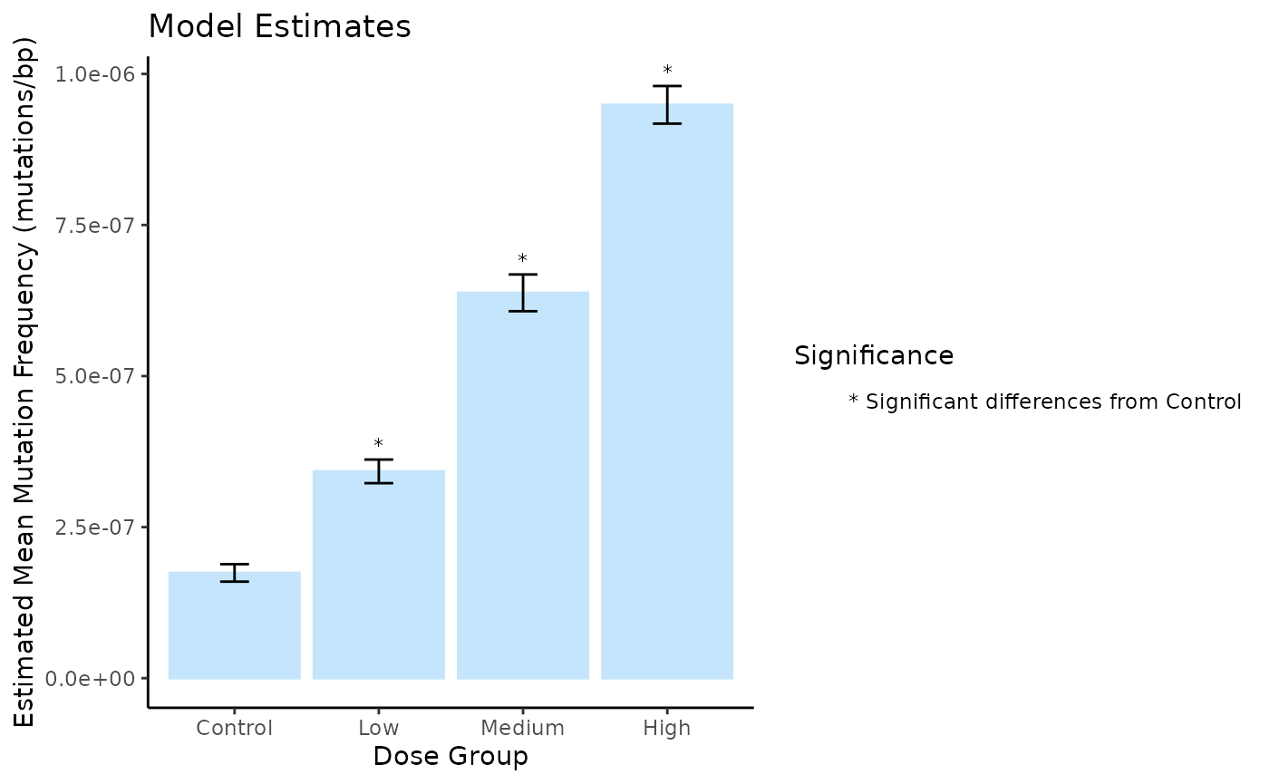

Mean Mutation Frequency Minimum (mutations/bp) per Dose estimated using a generalized linear model. Error bars are the S.E.M. Symbols indicate significance differences (p < 0.05).

Plot Model by Dose and Target

In this example, we only made comparisons between dose groups. For each contrast, we held the label (target) constant. Thus, we will set the ref_effect to dose_group so that significance labels are generated to indicate differences in dose, and not label.

# Define the order of the genomic targets for the x-axis:
# We will order them from lowest to highest MF at the High dose.
label_order <- model_by_target$point_estimates %>%
  dplyr::filter(dose_group == "High") %>%
  dplyr::arrange(Estimate) %>%
  dplyr::pull(label)

# Define the order of the doses for the fill
dose_order <- c("Control", "Low", "Medium", "High")

plot <- plot_model_mf(
  model = model_by_target,
  plot_type = "bar",
  x_effect = "label",
  plot_error_bars = TRUE,
  plot_signif = TRUE,
  ref_effect = "dose_group",
  x_order = label_order,
  fill_order = dose_order,
  x_label = "Target",
  y_label = "Mutation Frequency (mutations/bp)",
  fill_label = "Dose",
  plot_title = "",
  custom_palette = c("#ef476f",
                     "#ffd166",
                     "#06d6a0",
                     "#118ab2")
)
# Rotate the x-axis labels for clarity using ggplot2 functions.
plot <- plot + ggplot2::theme(axis.text.x = ggplot2::element_text(angle = 90))
plot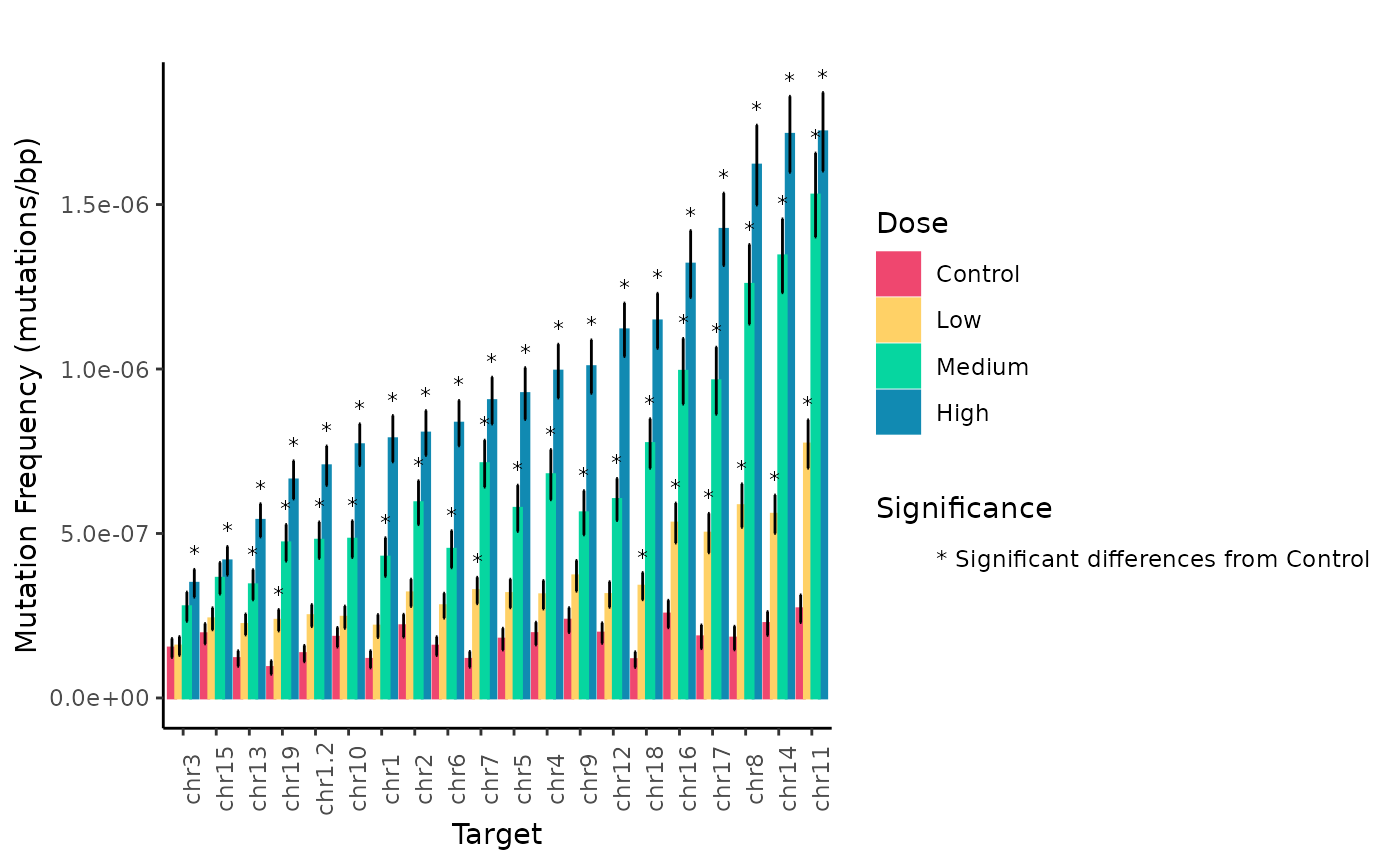

Mean Mutation Frequency Minimum (mutations/bp) per Genomic Target and Dose estimated using a generalized linear mixed model. Error bars are the SEM. Symbols indicate significance differences (p < 0.05) between dose levels for individual genomic regions.

These plots facilitate the interpretation of results. We can clearly see how MF varies based on the genomic target while increasing with dose.

Exporting Model Results

write_excel() will extract the mf_data, point_estimates, and pairwise_comparisons from model_mf() output to write to an excel workbook. To export model results, provide write_excel with the output of model_mf and set the model_results parameter to TRUE.

Example 3. Export model results

write_excel(
  model_by_dose,
  workbook_name = "Example_model",
  model_results = TRUE
)

Benchmark Dose Modeling

Dose-response models are essential for quatitative risk assessment of mutagenicity, as they provide a framework to evaluate the levels at which exposure to a substance might cause an adverse effect. The benchmark dose (BMD) is a dose that produces a predetermined change in the measured response, defined as the benchmark response (BMR). The BMD is used as a point of departure to derive human health-based guidance values to inform regulatory risk assessment such as the reference dose (RfD), the derived no-effect level (DNEL) or the acceptable daily intake (ADI) (Committee et al. 2022).

The BMD is estimated by applying various mathmatical models to fit the dose-response data. Some requirements must be met before modelling the BMD. There must be a clear dose-response trend in the MF data. We suggest using model_mf() to test for significant increases in MF with dose prior to running a BMD analysis. In general, studies with more dose groups and a graded monotonic response with dose will be more useful for BMD analysis. A minimum of three dose groups + 1 control group is suggested. Datasets in which a response is only observed at the high dose are usually not suitable for BMD modeling. However, if the one elevated response is near the BMR, adequate BMD computation may result. For a better estimate of the BMD, it is preferable to have studies with one or more doses near the level of the BMR.

Protection and safety authorities recommend the use of model averaging to determine the BMD and its confidence intervals. Model averaging incorporates information across multiple models to acount for model uncertainty, allowing the BMD to be more accurately estimated.

Ideally, the BMR would be based on a consensus scientific definition of what minimal level of change in MF is biologically significant. Currently, the default provided by this package calculates the BMD at a 50% relative increase in MF from the background. This BMR was selected based on previous recommendations for genotoxicity assessment by White, Long, and Johnson (2020).

MutSeqR provides bmd_proast for BMD modelling, which runs a modified version of the proast71.1 R library that is parametirized instead of menu-based.

bmd_proast will analyze the continuous, individual MF data following a log transformation. PROAST uses four families of nested models: exponential, Hill, inverse exponential, and log-normal. The Akaike information criterion (AIC) is used to select best fit. BMD confidence intervals are assessed by the Maximum Likelihood Profile method, or by model averaging via bootstrapping (recommended). BMR values are a user-defined relative increase in MF from the control. Alternatively, users may set the BMR as one standard-deviation from the control.

General Usage: bmd_proast

Supply bmd_proast with per-sample mf data calculated using calculate_mf(), with the dose column retained in the summary table. Dose column must be numeric.

Specify the column that contains the numeric dose values in dose_col. The function can model more than one response variable at once. Supply all response variables to response_col. If you wish to include a covariate in the analysis, supply the covariate variable to covariate_col. PROAST will assess if the BMD values differ significantly between levels of the covariate and give a BMD estimate for each.

It is highly recommended to use model averaging when calculating the BMD confidence intervals. Specify the number of bootstraps to run with num_bootstraps. The recommended value is 200, but be aware that this may take some time to run. PROAST model averaging will return the upper and lower 90% BMD confidence intervals. MutSeqR calculates the model-averaged BMD value as the median BMD of all bootstrap runs.

Users may choose to generate model plots with plot_results. Plots may be automatically saved to an output directory specified in output_path. Alternatively, when output_path is NULL, plots will automcatically be displayed and then returned within a list alongside the BMD summary results.

The function will output a data frame of final results, including a BMD estimate for each model family and the model averaging results, if applicable. Users may access the raw, unparsed PROAST results by setting raw_results = TRUE.

Example

Example 2.1. Calculate the BMD with model averaging for a 50% relative increase in MF from control. This will be calculated for both MFmin and MFmax. See the vignette to see information on how we imported and filtered the data.

Fist, calculate MF per sample while retaining the numeric dose column:

# load example data:
example_data <- eh[["EH9861"]]

mf_data_global <- calculate_mf(
  mutation_data = example_data,
  cols_to_group = "sample",
  subtype_resolution = "none",
  retain_metadata_cols = c("dose")
)

Next, run bmd_proast()

proast_results <- bmd_proast(
  mf_data = mf_data_global,
  dose_col = "dose",
  response_col = c("mf_min", "mf_max"),
  bmr = 0.5,
  model_averaging = TRUE,
  num_bootstraps = 10, # recommended value 200
  plot_results = TRUE,
  output_path = NULL
)

BMD Results

Summary

Table 22. BMD Estimates by PROAST.

We are mostly interested in the model averaging results. For MFmin, we would report that BaP induces a 50% increase in MF relative to controls at a dose of 9.11 mg/kg-bw/d (90% CI 8.39 - 9.87).

Exponential & Hill Models

replayPlot(proast_results$mf_min_Expon_HILL)

The fitted curve of the selected Exponenetial (left) and Hill (right) models. Data is MFmin by Dose following log-transformation. Individual data points are plotted using small triangles. The geometric mean at each dose is plotted as a large triangle. The estimated BMD is indicated by a dotted line.

replayPlot(proast_results$mf_max_Expon_HILL)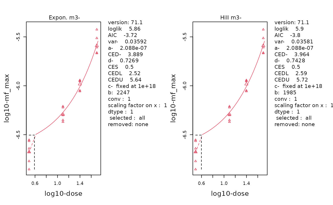

The fitted curve of the selected Exponenetial (left) and Hill (right) models. Data is MFmax by Dose following log-transformation. Individual data points are plotted using small triangles. The geometric mean at each dose is plotted as a large triangle. The estimated BMD is indicated by a dotted line.

Inverse Exponential & Log-Normal Models

replayPlot(proast_results$mf_min_InvExp_LN)

The fitted curve of the selected Inverse-Exponenetial (left) and Log-Normal (right) models. Data is MFmin by Dose following log-transformation. Individual data points are plotted using small triangles. The geometric mean at each dose is plotted as a large triangle. The estimated BMD is indicated by a dotted line.

replayPlot(proast_results$mf_max_InvExp_LN)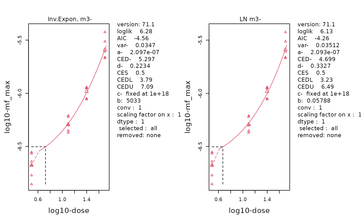

The fitted curve of the selected Inverse-Exponenetial (left) and Log-Normal (right) models. Data is MFmax by Dose following log-transformation. Individual data points are plotted using small triangles. The geometric mean at each dose is plotted as a large triangle. The estimated BMD is indicated by a dotted line.

Bootstrap Curves

replayPlot(proast_results$mf_max_bootstrap_curves)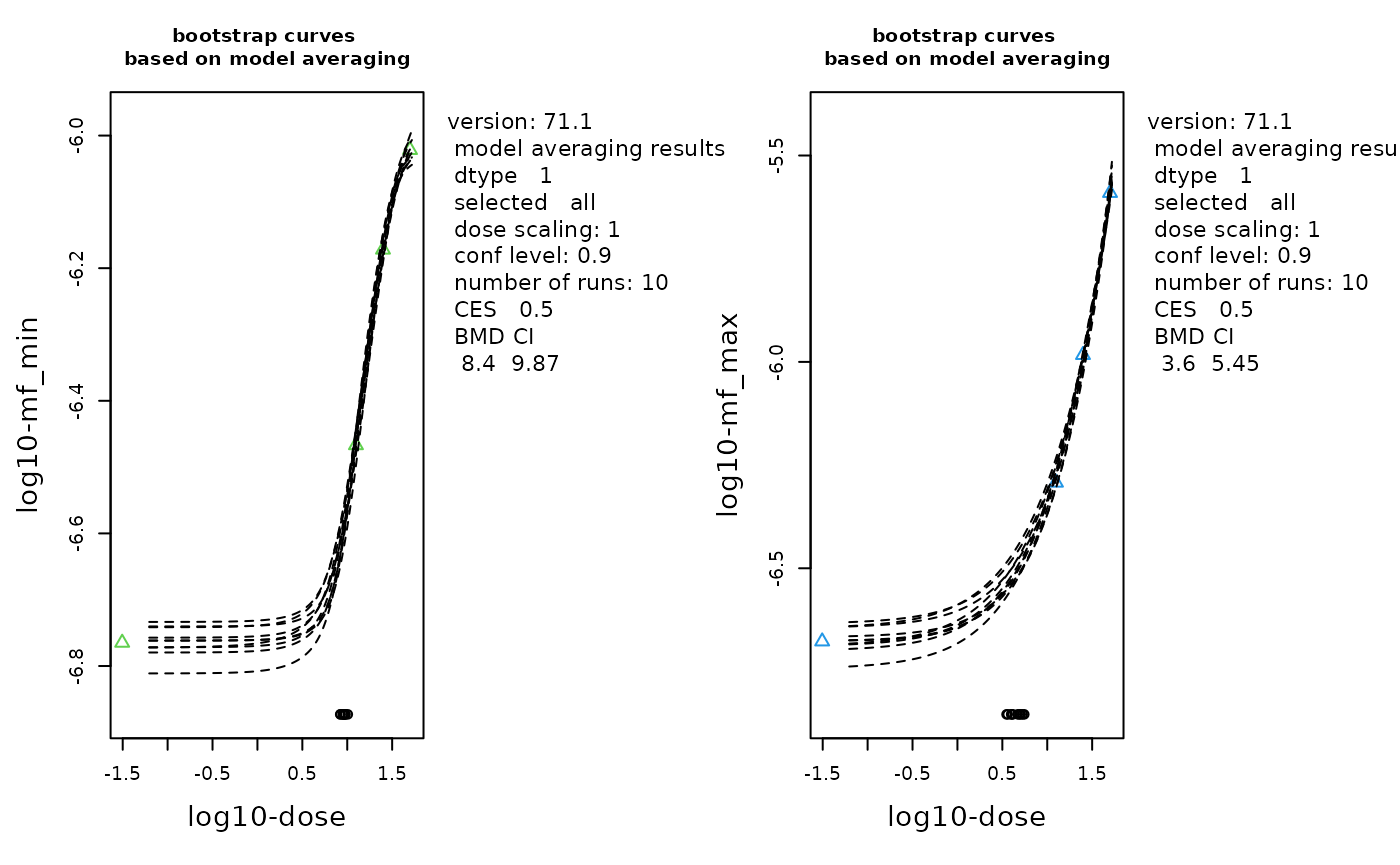

The bootstrap curves based on model averaging. Data is MFmin (left) and MFmax (right) by Dose with log-transformation. The geometric mean at each dose is plotted as a triangle. Number of bootstraps = 10 (although the recommended value is 200).

Cleveland Plots

proast_results$mf_min_cleveland

MFmin. The BMD estimate for each model plotted as a red point alongside the 90% confidence intervals. The size of the BMD point represents the model weight assigned during model averaging based on AIC.

proast_results$mf_max_cleveland

MFmax. The BMD estimate for each model plotted as a red point alongside the 90% confidence intervals. The size of the BMD point represents the model weight assigned during model averaging based on AIC.

Plot BMD CIs

plot_ci() creates a confidence interval (CI) plot of BMD results for easy comparison of BMDs between response variables.

The BMD values can be plotted on the log scale, if required.

Example 2.2. Compare the estimated BMD for MFmin (50% relative increase) by PROAST versus ToxicR (another BMD software available on Github,

calculated independently)*

plot_results <- data.frame(
  Response = c("PROAST", "ToxicR"),
  BMD = c(9.111, 9.641894),
  BMDL = c(7.38, 8.032936),
  BMDU = c(10.9, 10.97636)
)
plot <- plot_ci(
  data = plot_results,
  order = "asc",
  x_lab = "Dose (mg/kg-bw/d)",
  y_lab = "BMD Method"
)
plot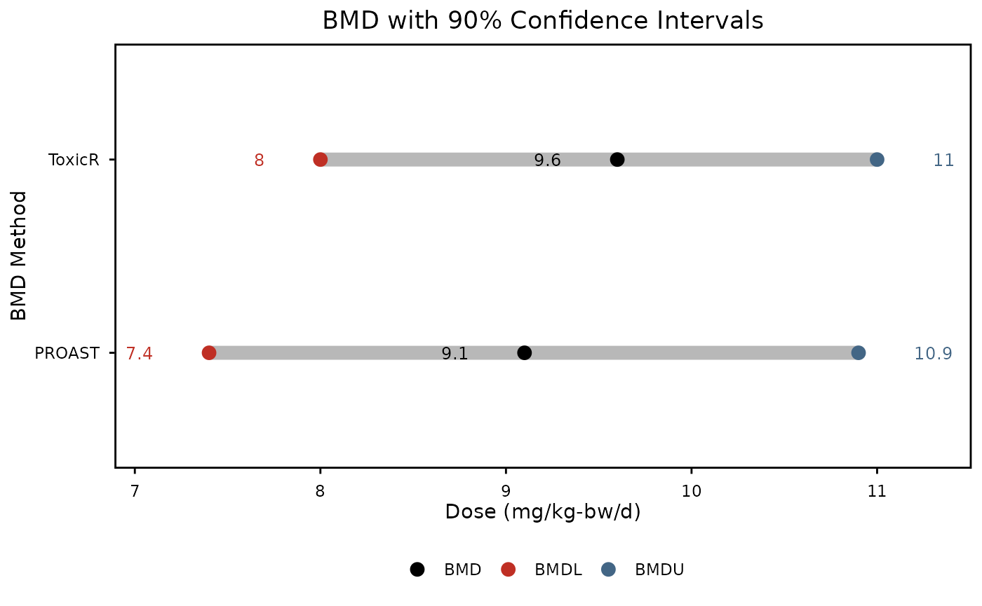

Benchmark dose with 90% confidence intervals representing the dose at, which a 50% increase in mutation frequency occurs from reference level. Calculated using ROAST software. Black points represent the BMD, red points the BMDL, and blue points, the BMDU

These plots are great for comparing BMDs between different groups. For our purposes, we see that PROAST and ToxicR generate BMD results that are pretty similar to each other. Since the confidence intervals are overlapping, we can say that the results from the two BMD software tools are not statistically different from each other. These plots would also be great for comparing the potency of different chemicals.

References

Appendix

Session Info

## R Under development (unstable) (2025-11-18 r89035)
## Platform: x86_64-pc-linux-gnu
## Running under: Ubuntu 24.04.3 LTS
## 
## Matrix products: default
## BLAS:   /usr/lib/x86_64-linux-gnu/openblas-pthread/libblas.so.3 
## LAPACK: /usr/lib/x86_64-linux-gnu/openblas-pthread/libopenblasp-r0.3.26.so;  LAPACK version 3.12.0
## 
## locale:
##  [1] LC_CTYPE=C.UTF-8       LC_NUMERIC=C           LC_TIME=C.UTF-8       
##  [4] LC_COLLATE=C.UTF-8     LC_MONETARY=C.UTF-8    LC_MESSAGES=C.UTF-8   
##  [7] LC_PAPER=C.UTF-8       LC_NAME=C              LC_ADDRESS=C          
## [10] LC_TELEPHONE=C         LC_MEASUREMENT=C.UTF-8 LC_IDENTIFICATION=C   
## 
## time zone: UTC
## tzcode source: system (glibc)
## 
## attached base packages:
## [1] stats     graphics  grDevices utils     datasets  methods   base     
## 
## other attached packages:
##  [1] ExperimentHub_3.1.0 AnnotationHub_4.1.0 BiocFileCache_3.1.0
##  [4] dbplyr_2.5.1        BiocGenerics_0.57.0 generics_0.1.4     
##  [7] MutSeqR_0.99.3      yulab.utils_0.2.1   htmltools_0.5.8.1  
## [10] DT_0.34.0          
## 
## loaded via a namespace (and not attached):
##   [1] Rdpack_2.6.4                DBI_1.2.3                  
##   [3] bitops_1.0-9                httr2_1.2.1                
##   [5] rlang_1.1.6                 magrittr_2.0.4             
##   [7] matrixStats_1.5.0           compiler_4.6.0             
##   [9] RSQLite_2.4.4               GenomicFeatures_1.63.1     
##  [11] png_0.1-8                   systemfonts_1.3.1          
##  [13] vctrs_0.6.5                 stringr_1.6.0              
##  [15] pkgconfig_2.0.3             crayon_1.5.3               
##  [17] fastmap_1.2.0               backports_1.5.0            
##  [19] XVector_0.51.0              labeling_0.4.3             
##  [21] Rsamtools_2.27.0            rmarkdown_2.30             
##  [23] nloptr_2.2.1                ragg_1.5.0                 
##  [25] purrr_1.2.0                 bit_4.6.0                  
##  [27] xfun_0.54                   cachem_1.1.0               
##  [29] cigarillo_1.1.0             jsonlite_2.0.0             
##  [31] blob_1.2.4                  DelayedArray_0.37.0        
##  [33] BiocParallel_1.45.0         Deriv_4.2.0                
##  [35] broom_1.0.10                parallel_4.6.0             
##  [37] R6_2.6.1                    plyranges_1.31.1           
##  [39] VariantAnnotation_1.57.0    bslib_0.9.0                
##  [41] stringi_1.8.7               RColorBrewer_1.1-3         
##  [43] rtracklayer_1.71.0          car_3.1-3                  
##  [45] boot_1.3-32                 GenomicRanges_1.63.0       
##  [47] jquerylib_0.1.4             Rcpp_1.1.0                 
##  [49] Seqinfo_1.1.0               SummarizedExperiment_1.41.0
##  [51] knitr_1.50                  modelr_0.1.11              
##  [53] IRanges_2.45.0              splines_4.6.0              
##  [55] Matrix_1.7-4                tidyselect_1.2.1           
##  [57] dichromat_2.0-0.1           abind_1.4-8                
##  [59] yaml_2.3.10                 codetools_0.2-20           
##  [61] curl_7.0.0                  lattice_0.22-7             
##  [63] tibble_3.3.0                Biobase_2.71.0             
##  [65] withr_3.0.2                 KEGGREST_1.51.1            
##  [67] S7_0.2.1                    evaluate_1.0.5             
##  [69] desc_1.4.3                  Biostrings_2.79.2          
##  [71] pillar_1.11.1               BiocManager_1.30.27        
##  [73] filelock_1.0.3              carData_3.0-5              
##  [75] MatrixGenerics_1.23.0       stats4_4.6.0               
##  [77] reformulas_0.4.2            rprojroot_2.1.1            
##  [79] RCurl_1.98-1.17             BiocVersion_3.23.1         
##  [81] S4Vectors_0.49.0            ggplot2_4.0.1              
##  [83] scales_1.4.0                minqa_1.2.8                
##  [85] glue_1.8.0                  tools_4.6.0                
##  [87] doBy_4.7.0                  BiocIO_1.21.0              
##  [89] data.table_1.17.8           lme4_1.1-37                
##  [91] BSgenome_1.79.1             GenomicAlignments_1.47.0   
##  [93] fs_1.6.6                    XML_3.99-0.20              
##  [95] cowplot_1.2.0               grid_4.6.0                 
##  [97] tidyr_1.3.1                 rbibutils_2.4              
##  [99] crosstalk_1.2.2             AnnotationDbi_1.73.0       
## [101] nlme_3.1-168                restfulr_0.0.16            
## [103] Formula_1.2-5               cli_3.6.5                  
## [105] rappdirs_0.3.3              textshaping_1.0.4          
## [107] S4Arrays_1.11.0             ggdendro_0.2.0             
## [109] dplyr_1.1.4                 gtable_0.3.6               
## [111] sass_0.4.10                 digest_0.6.39              
## [113] SparseArray_1.11.2          rjson_0.2.23               
## [115] htmlwidgets_1.6.4           farver_2.1.2               
## [117] memoise_2.0.1               pkgdown_2.2.0              
## [119] lifecycle_1.0.4             httr_1.4.7                 
## [121] here_1.0.2                  microbenchmark_1.5.0       
## [123] bit64_4.6.0-1               MASS_7.3-65

Committee, EFSA Scientific, Simon John More, Vasileios Bampidis, Diane Benford, Claude Bragard, Thorhallur Ingi Halldorsson, Antonio F Hernández-Jerez, et al. 2022. “Guidance on the Use of the Benchmark Dose Approach in Risk Assessment.” EFSA Journal 20 (10): e07584. https://doi.org/10.2903/j.efsa.2022.7584.

White, Paul A., Alexandra S. Long, and George E. Johnson. 2020. “Quantitative Interpretation of Genetic Toxicity Dose‐Response Data for Risk Assessment and Regulatory Decision‐Making: Current Status and Emerging Priorities.” Environmental and Molecular Mutagenesis 61 (1): 66–83. https://doi.org/10.1002/em.22351.

Annette E. Dodge

Matthew J. Meier

Load MutSeqR and Example Data

Generalized Linear Modeling

Model Formula

Family

Estimates & Comparisons

Goodness of Fit

General Usage

Output

Examples

Example 1. Model by Dose

Residuals Histogram

Residuals QQ-plot

Model Summary

Model Estimates

Pairwise Comparisons

Example 2. Model by Dose and Target

Residuals Histogram

Residuals QQ-plot

Model Summary

ANOVA

Model Estimates

Pairwise Comparisons

Plot Model Results

Plot Model by Dose

Plot Model by Dose and Target

Exporting Model Results

Benchmark Dose Modeling

General Usage: bmd_proast

Example

BMD Results

Summary

Exponential & Hill Models

Inverse Exponential & Log-Normal Models

Bootstrap Curves

Cleveland Plots

Plot BMD CIs

References

Appendix

Session Info