MutSeqR: Error-Corrected Sequencing (ECS) Analysis For Mutagenicity Assessment

Annette E. Dodge

Environmental Health Science and Research Bureau, Health Canada, Ottawa, ON, Canada.

Matthew J. Meier

matthew.meier@hc-sc.gc.ca

Introduction

In this module we will provide instructions on how to import, filter, and summarize mutation data generated by Error-correct next-generation sequencing (ECS). For information on how to use MutSeqR for statistical analysis of the data, see the relevant modules:

• Modelling Mutation Frequencies (Generalized Linear Modelling and BMD)
• Analyzing Mutation Spectra (Comparison of Spectra and Mutation Signature Analysis)
• Target Analysis
• Other Features (visualization of clonal mutations, retrieve target sequences)

What is ECS?

Error-corrected next-generation sequencing (ECS) uses various methods to combine multiple independent raw sequence reads derived from an original starting molecule, thereby subtracting out artifacts introduced during sequencing or library preparation. This results in a highly accurate representation of the original molecule. ECS is particularly useful for detecting rare somatic mutations (or mutations induced in germ cells), such as those that arise from mutagen exposure or other sources of DNA damage. ECS is a powerful tool for assessing the mutagenicity of chemicals, drugs, or other agents, and can be used to identify the mutational signatures of these agents. ECS can also be used to detect rare mutations in cancer or other diseases, and to track the clonal evolution of these diseases over time.

For more background on how ECS works and its context in regulatory toxicology testing and genetic toxicology, see the following articles:

• Menon and Brash (2023)
• Marchetti, Cardoso, Chen, Douglas, Elloway, Escobar, Harper, et al. (2023)
• Marchetti, Cardoso, Chen, Douglas, Elloway, Escobar, Harper Jr, et al. (2023)
• Kennedy et al. (2014)

This R package is meant to facilitate the import, cleaning, and analysis of ECS data, beginning with a table of variant calls or a variant call file (VCF). The package is designed to be flexible and enable users to perform common statistical analyses and visualisations.

Installation

Install the package from Bioconductor:

if (!require("BiocManager", quietly = TRUE)) {
  install.packages("BiocManager")
}
BiocManager::install("MutSeqR")

Load the package

library(MutSeqR)

Data import

The main goal of MutSeqR is to generate summary statistics, visualizations, exploratory analyses, and other post-processing tasks such as mutational signature analysis or generalized linear modeling. Mutation data should be supplied as a table of variants with their genomic positions. Mutation data can be imported as either VCF files or as tabular data using the functions import_vcf_data and import_mut_data, respectively. It is reccomended that files include a record for every sequenced position, regardless of whether a variant was called or not, along with the total_depth for each record. This enables site-specific depth calculations that are required for the calculation of mutation subtype frequencies and other site-specific frequencies. The data set can be pared down later to include only mutations of interest (SNVs, indels, SVs, or any combination).

(#tab:required-columns) Required columns for mutation data import.

Column	VCF Specification	Definition
contig	CHROM	The name of the reference sequence.
start	POS	The start position of the feature. 0-based coordinates are accepted but will be changed to 1-based during import.
end	INFO(END)	The half-open end position of the feature in contig.
ref	REF	The reference allele at this position.
alt	ALT	The left-aligned, normalized, alternate allele at this position.
sample	INFO(sample) or Genotype Header	A unique identifier for the sample library. For VCF files, this field may be provided in either the INFO field, or as the header to the GENOTYPE field.
SUGGESTED FIELDS
alt_depth	VD	The read depth supporting the alternate allele. If not included, the function will assume an alt_depth of 1 at variant sites.
total_depth or depth	AD or DP	The total read depth at this position. This column can be “total_depth” which excludes N-calls, or “depth”, which includes N-calls, if “total_depth” is not available. For VCF files, the total_depth is calculated as the sum of AD. DP is equivalent to “depth”.

VCF files should follow the VCF specification (version 4.5; Danecek et al. (2011)). VCF files may be bg/g-zipped. Each individual VCF file should contain the mutation data for a single sample library. Multiple alt alleles called for a single position should be represented as separate rows in the data. All extra columns, INFO fields, and FORMAT fields will be retained upon import.

Upon import, records are categorized within the variation_type column based on their REF and ALT. Categories are listed below.

(#tab:variation-types) Definitions of Variation types.

variation_type	Definition
no_variant	No variation, the null-case.
snv	Single nucleotide variant.
mnv	Multiple nucleotide variant.
insertion	Insertion.
deletion	Deletion.
complex	REF and ALT are of different lengths and nucleotide compositions.
symbolic	Structural variant
ambiguous	ALT contains IUPAC ambiguity codes.
uncategorized	The record does not fall into any of the preceding categories.

Additional columns are created to further characterise variants.

(#tab:mut-columns) Definitions of Mutation data columns.

Column Name	Definition
short_ref	The reference base at the start position.
normalized_ref	The short_ref in C/T (pyrimidine) notation for this position. Ex. A -> T, G -> C
context	The trinucleotide context at this position. Consists of the reference base and the two flanking bases. Sequences are retrieved from the appropriate BS genome. Ex. TAC
normalized_context	The trinucleotide context in C/T (pyrimidine) notation for this position (Ex. TAG -> CTA)
variation_type	The type of variant (no_variant, snv, mnv, insertion, deletion, complex, sv, ambiguous, uncategorized)
subtype	The substitution type of the snv variant (12-base spectrum; Ex. A>C)
normalized_subtype	The snv subtype in C/T (pyrimidine) notation (6-base spectrum; Ex. A>C -> T>G)
context_with_mutation	The snv subtype including the two flanking nucleotides (192-base spectrum; Ex. T[A>C]G)
normalized_context_with_mutation	The snv subtype in C/T (pyrimidine) notation including the two flanking nucleotides (96-base spectrum; Ex. T[A>C]G -> C[T>G]A)
nchar_ref	The length (in bp) of the reference allele.
nchar_alt	The length (in bp) of the alternate allele.
varlen	The length (in bp) of the variant.
ref_depth	The depth of the reference allele. Calculated as total_depth - alt_depth, if applicable.
vaf	The variant allele fraction. Calculated as alt_depth/total_depth
gc_content	% GC of the trinucleotide context at this position.
is_known	A logical value indicating if the record is a known variant; i.e. ID field is not NULL.
row_has_duplicate	A logical value that flags rows whose position is the same as that of at least one other row for the same sample.

General Usage

Indicate the filepath to your mutation data file(s) using the vcf_file/ mut_file parameter. This can be either a single file or a directory containing multiple files. Should you provide a directory, then all files within will be bound into a single data frame.

An important component of importing your data for proper use is to assign each mutation to a biological sample, and also make sure that some additional information about each sample is present (ex., a chemical treatment, a dose, etc.). This is done by providing sample_data. This parameter can take a data frame, or it can read in a file if provided it with a filepath. If using a filepath, specify the proper delimiter using the sd_sep parameter. Sample metadata will be joined with the mutation data using the “sample” column to capture that information and associate it with each mutation.

Specify the appropriate BS genome with which to populate the context column. Prior to data import, ensure that the BS genome is installed. Supply the pkgname to the BS_genome parameter in the import function. If you are not sure which BS genome you should use, you can use the find_BS_genome() function. This function will browse BSgenome::available.genomes for given organisms and genome assembly versions. Once you’ve identified the appropriate BS genome, it can be installed using BiocManager(). Context information will be extracted from the BS genome. Note, BSgenome offers genomes with masked sequences. If you wish to use the masked version of the genome, you can find the right one with find_BS_genome(masked = TRUE).

Examples

We provide an example data set taken from LeBlanc et al. (2022). This data consists of 24 mouse bone marrow samples sequenced with Duplex Sequencing using Twinstrand’s Mouse Mutagenesis Panel of twenty 2.4kb targeted genomic loci. Mice were exposed to three doses of benzo[a]pyrene (BaP) alongside vehicle controls, n = 6. Example data is retrieved from MutSeqRData, an ExperimentHub data package available via Bioconductor. Example data can be retrieved from the ExperimentHub index (eh) through specific accessors.

library(ExperimentHub)
# load the index
eh <- ExperimentHub()
# Query the index for MutSeqRData records and their associated accessors.
query(eh, "MutSeqRData")

## ExperimentHub with 9 records
## # snapshotDate(): 2025-11-14
## # $dataprovider: Health Canada, TwinStrand Biosciences
## # $species: Mus musculus
## # $rdataclass: data.frame
## # additional mcols(): taxonomyid, genome, description,
## #   coordinate_1_based, maintainer, rdatadateadded, preparerclass, tags,
## #   rdatapath, sourceurl, sourcetype 
## # retrieve records with, e.g., 'object[["EH9857"]]' 
## 
##            title                                            
##   EH9857 | Example import_mut_data                          
##   EH9858 | Example import_mut_data using Custom column names
##   EH9859 | Example import_vcf_data                          
##   EH9860 | Example mutation data                            
##   EH9861 | Example mutation data filtered                   
##   EH9862 | Precalculated Depth at Base 6 Resolution         
##   EH9863 | Precalculated Depth at Base 12 Resolution        
##   EH9864 | Precalculated Depth at Base 96 Resolution        
##   EH9865 | Precalculated Depth at Base 192 Resolution

Identify the BS genome: Sequencing data was aligned to the mm10 mouse genome.

mouse_BS_genome <- find_BS_genome(organism = "mouse", genome = "mm10")
print(mouse_BS_genome)

## [1] "BSgenome.Mmusculus.UCSC.mm10"

Install the appropriate BS genome:

BiocManager("BSgenome.Mmusculus.UCSC.mm10")

VCF

Example 1.1. Import the example .vcf.bgz file “Example import_vcf_data”. Provided is the genomic vcf.gz file for sample dna00996.1. It is comprised of a record for all 48K positions sequenced for the Mouse Mutagenesis Panel with the alt_depth and the tota_depth values for each record.

example_file <- eh[["EH9859"]]

sample_metadata <- data.frame(
  sample = "dna00996.1",
  dose = "50",
  dose_group = "High"
)
# Import the data
imported_example_data <- import_vcf_data(
  vcf_file = example_file,
  sample_data = sample_metadata,
  BS_genome = mouse_BS_genome
)

Data Table 1. Mutation data imported from VCF for sample dna00996.1. Displays the first 6 rows.

Tabular

Example 1.2. Import example tabular data “Example import_mut_data”. This is the equivalent file to the example vcf file. It is stored as an .rds file. We will load the dataframe and supply it to import_mut_data. The mut_file parameter can accept file paths or data frames as input.

example_data <- eh[["EH9857"]]

sample_metadata <- data.frame(
  sample = "dna00996.1",
  dose = "50",
  dose_group = "High"
)
# Import the data
imported_example_data <- import_mut_data(
  mut_file = example_data,
  sample_data = sample_metadata,
  BS_genome = find_BS_genome("mouse", "mm10"), # Must be installed!!
  is_0_based_mut = TRUE # indicates that the genomic coordinates are 0-based.
# Coordinates will be changed to 1-based upon import.
)

Data Table 2. Mutation data imported from a data.frame object for sample dna00996.1. Displays the first 6 rows.

Region Metadata

Similar to sample metadata, you may supply a file containing the metadata of genomic regions to the regions parameter. In the file, the genomic regions are defined by the name of their reference sequence plus their start and end coordinates. Additional columns are added to describe features of the genomic regions (Ex. transcription status, GC content, etc.). Region metadata will be joined with mutation data by checking for overlap between the target region ranges and the position of the record. The regions parameter can be either a filepath, a data frame, or a GRanges object. Filepaths will be read using the rg_sep. Users can also choose from the built-in TwinStrand DuplexSeq™ Mutagenesis Panels by inputting “TSpanel_human”, “TSpanel_mouse”, or “TSpanel_rat”. Required columns for the regions file are “contig”, “start”, and “end”. In a GRanges object, the required columns are “seqnames”, “start”, and “end”. Users must indicate whether the region coordinates are 0-based or 1-based with is_0_based_rg. Mutation data and region coordinates will be converted to 1-based. If you do not wish to specify regions, then set the regions parameter to NULL (default).

Example 1.3. Add the metadata for TwinStrand’s Mouse Mutagenesis panel to our example tabular file.

imported_example_data <- import_mut_data(
  mut_file = example_data,
  sample_data = sample_metadata,
  BS_genome = find_BS_genome("mouse", "mm10"),
  is_0_based_mut = TRUE,
  regions = "TSpanel_mouse"
)

Data Table 3. Mutation data imported from a data.frame object for sample dna00996.1 with added metadata for the Mouse Mutagenesis Panels sequencing targets. Displays the first 6 rows. Added columns are ‘target_size’, ‘label’, ‘genic_context’, ‘region_GC_content’, ‘genome’, and ‘in_regions’.

Users can load the example TwinStrand Mutagenesis Panels with load_regions(). This function will output a GRanges object. Custom panels may also be loaded with this function by providing their file path to the regions parameter.

region_example <- load_regions_file("TSpanel_mouse")
region_example

## GRanges object with 20 ranges and 5 metadata columns:
##        seqnames              ranges strand | target_size       label
##           <Rle>           <IRanges>  <Rle> |   <integer> <character>
##    [1]     chr1   69304218-69306617      * |        2400        chr1
##    [2]     chr1 155235939-155238338      * |        2400      chr1.2
##    [3]     chr2   50833176-50835575      * |        2400        chr2
##    [4]     chr3 109633161-109635560      * |        2400        chr3
##    [5]     chr4   96825281-96827680      * |        2400        chr4
##    ...      ...                 ...    ... .         ...         ...
##   [16]    chr15   66779763-66782162      * |        2400       chr15
##   [17]    chr16   72381581-72383980      * |        2400       chr16
##   [18]    chr17   94009029-94011428      * |        2400       chr17
##   [19]    chr18   81262079-81264478      * |        2400       chr18
##   [20]    chr19     4618814-4621213      * |        2400       chr19
##        genic_context region_GC_content      genome
##          <character>         <numeric> <character>
##    [1]    intergenic              37.3        mm10
##    [2]         genic              54.0        mm10
##    [3]    intergenic              45.3        mm10
##    [4]         genic              39.2        mm10
##    [5]    intergenic              39.4        mm10
##    ...           ...               ...         ...
##   [16]         genic              44.0        mm10
##   [17]    intergenic              38.3        mm10
##   [18]    intergenic              35.2        mm10
##   [19]    intergenic              47.3        mm10
##   [20]         genic              56.1        mm10
##   -------
##   seqinfo: 19 sequences from an unspecified genome; no seqlengths

Custom Column Names

We recognize that column names may differ from those specified in Table @ref(tab:required-columns). Therefore, we have implemented some default column name synonyms. If your column name matches one of our listed synonyms, it will automatically be changed to match our set values. For example, your contig column may be named chr or chromosome. After importing your data, this synonymous column name will be changed to contig. Column names are case-insensitive. A list of column name synonyms are listed below.

(#tab:name-sym) Predefined column name synonyms. Synonyms will be automatically changed to the default Column value upon import.

Column	Synonyms
alt	alternate
alt_depth	alt_read_depth, var_depth, variant_depth, vd
context	sequence_context, trinucleotide_context, flanking_sequence
contig	chr, chromosome, seqnames
depth	dp
end	end_position
no_calls	n_calls, n_depth, no_depth
ref	reference, ref_value
sample	sample_name, sample_id
start	pos, position
total_depth	informative_somatic_depth

If your data contains a column that is synonymous to one of the required columns, but the name is not included in our synonyms list, your column name may be substituted using the custom_column_names parameter. Provide this parameter with a list of names to specify the meaning of column headers.

mut_data <- eh[["EH9858"]]

## MutSeqRData not installed.
##   Full functionality, documentation, and loading of data might not be possible without installing

## downloading 1 resources

## retrieving 1 resource

## loading from cache

imported_example_data_custom <- import_mut_data(
  mut_file = mut_data,
  custom_column_names = list(my_contig_name = "contig",
                             my_sample_name = "sample")
)

## 'getOption("repos")' replaces Bioconductor standard repositories, see
## 'help("repositories", package = "BiocManager")' for details.
## Replacement repositories:
##     CRAN: https://cran.rstudio.com

## Expected 'contig' but found 'my_contig_name', renaming it.

## Expected 'sample' but found 'my_sample_name', renaming it.

Data Table 4. Mutation data imported from tabular file with custom column names. Displays the first 6 rows. Custom column names are changed to default values.

Output

Mutation data can be output as either a data frame or a GRanges object for downstream analysis. Use the output_granges parameter to specify the output. GRanges may faciliate use in other packages and makes doing genomic based analyses on the ranges significantly easier. Most downstream analyses provided by MutSeqR will use a data frame.

Variant Filtering

Following data import, the mutation data may be filtered using the filter_mut() function. This function will flag variants based on various parameters in the filter_mut column. Variants flagged as TRUE in the filter_mut column will be automatically excluded from downstream analyses such as calculate_mf(), plot_bubbles, and signature_fitting. When specified, this function may also remove records from the mutation data.

Flagging the variants in the filter_mut column will not remove them from the mutation data, however, they will be excluded from mutation counts in all downstream analyses. Filtered variants are retained in the data so that their total_depth values may still be used in frequency calculations.

By default, all filtering parameters are disabled. Users should be mindful of the filters that they use, ensuring first that they are applicable to their data.

Germline Variants

Germline variants may be identified and flagged for filtering by setting the vaf_cutoff parameter. The variant allele fraction (vaf) is the fraction of haploid genomes in the original sample that harbor a specific mutation at a specific base-pair coordinate of the reference genome. Specifically, is it calculated by dividing the number of variant reads by the total sequencing depth at a specific base pair coordinate (alt_depth / total_depth). In a typical diploid cell, a homozygous germline variant will appear on both alleles, in every cell. As such, we expect this variant to occur on every read, giving us a vaf = 1. A heterozygous germline variant occurs on one of the two alleles in every cell, as such we expect this variant to occur on about half of the reads, giving a vaf = 0.5. Somatic variants occur in only a small portion of the cells, thus we expect them to appear in only a small percentage of the reads. Typical vaf values for somatic variants are less than 0.01 - 0.1. Setting the vaf_cutoff parameter will flag all variants that have a vaf greater than this value as germline within the is_germline column. It will also flag these variants in the filter_mut so as to exclude them from downstream analyses.

vaf germline filtering is only applicable to users whose data was sequenced to a sufficient depth. High coverage/low depth sequencing cannot be used to calculate the vaf, thus it is recommended to filter germline mutations by contrasting against a database of known polymorphisms, or by using conventional whole-genome sequencing to identify germline variants for each sample.

Quality Assurance

The filter_mut() function offers some filtering options to ensure the quality of the mutation data.

snv_in_germ_mnv = TRUE will flag all snvs that overlap with germline mnvs. Germline mnvs are defined as having a vaf > vaf_cutoff. These snvs are often artifacts from variant calling. No-calls in reads supporting the germline mnv will create false minor-haplotypes from the original mnv that can appear as sub-clonal snvs, thus such variants are excluded from downstream analyses.

rm_abnormal_vaf = TRUE This parameter identifies rows with abnormal vaf values and removes them from the mutation data. Abnormal vaf values are defined as being between 0.05-0.45 or between 0.55-0.95. In a typical diploid organism, we expect variants to have a vaf ~0, 0.5, or 1, reflecting rare somatic variants, heterozygous variants, and homozygous variants respectively. Users should be aware of the ploidy of their model system when using this filter. Non-diploid organisms may exhibit different vafs.

rm_filtered_mut_from_depth = TRUE Variants flagged in the filter_mut column will have their alt_depth subtracted from the total_depth. When TRUE, this parameter treats flagged variants as No-calls. This does not apply to variants that were idenfied as germline variants.

Custom Filtering

Users may use the filter_mut() function to flag or remove variants based on their own custom column. Any record that contains the custom_filter_val value within the custom_filter_col column of the mutation data will be either flagged in the filter_mut column or, if specified by the custom_filter_rm parameter, removed from the mutation data.

Filtering by Regions

Users may remove rows that are either within or outside of specified genomic regions. Provide the region ranges to the regions parameter. This may be provided as either a filepath, data frame, or a GRanges object. regions must contain contig (or seqnames for GRanges), start, and end. The function will check whether each record falls within the given regions. Users can define how this filter should be used with regions_filter. region_filter = "remove_within" will remove all rows whose positions overlap with the provided regions. region_filter = "keep_within" will remove all rows whose positions are outside of the provided regions. By default, records that are

1bp must start and end within the regions to count as being within the region. allow_half_overlap = TRUE allow records that only start or end within the regions but extend outside of them to be counted as being within the region. Twinstrand Mutagenesis Panels may be used by setting regions to one of “TSpanel_human”, “TSpanel_mouse”, or “TSpanel_rat”.

Output

The function will return the mutation data as a data.frame object with rows removed or flagged depending on input parameters. Added columns are ‘filter_mut’, ‘filter_reason’, ‘is_germline’, and ‘snv_mnv_overlaps’. If return_filtered_rows = TRUE The function will return both the data.frame containing the processed mutation data and a data.frame containing the rows that were removed/flagged during the filtering process. The two dataframes will be returned inside of a list, with names mutation_data and filtered_rows. The function will also print the number of mutations/rows that were filtered according to each parameter.

Example

Example 2. The example file “Example mutation data” is the output of _import_mut_data() run on all 24 mouse libraries from (leblanc-2022._?)

Filters used:

• Filter germline variants: vaf < 0.01
• Filter snvs overlapping with germline variants and have their alt_depth removed from their total_depth.
• Remove records outside of the TwinStrand Mouse Mutagenesis Panel.
• Filter variants that contain “EndRepairFillInArtifact” in the “filter” column. Their alt_depth will be removed from their total_depth.

# load the example data
example_data <- eh[["EH9860"]]

## MutSeqRData not installed.
##   Full functionality, documentation, and loading of data might not be possible without installing

## downloading 1 resources

## retrieving 1 resource

## loading from cache

# Filter
filtered_example_mutation_data <- filter_mut(
  mutation_data = example_data,
  vaf_cutoff = 0.01,
  regions = "TSpanel_mouse",
  regions_filter = "keep_within",
  custom_filter_col = "filter",
  custom_filter_val = "EndRepairFillInArtifact",
  custom_filter_rm = FALSE,
  snv_in_germ_mnv = TRUE,
  rm_filtered_mut_from_depth = TRUE,
  return_filtered_rows = FALSE
)

## Flagging germline mutations...

## Found 612 germline mutations.

## Flagging SNVs overlapping with germline MNVs...

## Found 20 SNVs overlapping with germline MNVs.

## Applying custom filter...

## Flagged 2021 rows with values in <filter> column that matched EndRepairFillInArtifact

## Applying region filter...

## Removed 22 rows based on regions.

## Removing filtered mutations from the total_depth...

## Filtering complete.

Data Table 5. Filtered Mutation data for all 24 samples. Displayed are 6 variants that were flagged during filtering.

Calculating MF

Mutation Frequency (MF) is calculated by dividing the sum of mutations by the sum of the total_depth for a given group (units mutations/bp). The function calculate_mf() sums mutation counts and total_depth across user-defined groupings within the mutation data to calculate the MF. Mutations can be summarised across samples, experimental groups, and mutation subtypes for later statistical analyses. Variants flagged as TRUE in the filter_mut column will be excluded from the mutation sums; however, the total_depth of these variants will be counted in the total_depth sum.

If the total_depth is not available, the function will sum the mutations across groups, without calculating the mutation frequencies.

Mutation Counting

Mutations are counted based on two opposing assumptions (Dodge et al. 2023):

The Minimum Independent Mutation Counting Method (min) Each mutation is counted once, regardless of the number of reads that contain the non-reference allele. This method assumes that multiple instances of the same mutation within a sample are the result of clonal expansion of a single mutational event. When summing mutations across groups using the Min method (sum_min), the alt_depth of each variant is set to 1. Ex. For 3 variants with alt_depth values of 1, 2, and 10, the sum_min= 3.

The Maximum Independent Mutation Counting Method (max) Multiple identical mutations at the same position within a sample are counted as independent mutation events. When summing mutations across groups using the Max method (sum_max), the alt_depth of each variant is summed unchanged. Ex. for 3 variants with alt_depth values of 1, 2, and 10, the sum_max = 13.

The Min and Max mutation counting methods undercount and overcount the mutations, respectively. We expect some recurrent mutations to be a result of clonal expansion. We also expect some recurrent mutations to arise independently of each other. As we expect the true number of independent mutations to be somewhere in the middle of the two counting methods, we calculate frequencies for both methods. However, the Min mutation counting method is generally recommended for statistical analyses to ensure independance of values and because the Max method tends to increase the sample variance by a significant degree.

Grouping Mutations

Mutation counts and total_depth are summed across groups that can be designated using the cols_to_group parameter. This parameter can be set to one or more columns in the mutation data that represent experimental variables of interest.

Example 3.1. Calculate mutation sums and frequencies per sample. The file “Example mutation data filtered” is the output of filter_mut() from Example 2

# load example data:
example_data <- eh[["EH9861"]]

mf_data_global <- calculate_mf(
  mutation_data = example_data,
  cols_to_group = "sample",
  subtype_resolution = "none",
  retain_metadata_cols = c("dose_group", "dose")
)

Table 6. Global Mutation Frequency per Sample

Alternatively, you can sum mutations by experimental groups such as label (the genomic target). Counts and frequencies will be returned for every level of the designated groups.

Example 3.2. Calculate mutation sums and frequencies per sample and genomic target.

mf_data_rg <- calculate_mf(
  mutation_data = example_data,
  cols_to_group = c("sample", "label"),
  subtype_resolution = "none",
  retain_metadata_cols = "dose_group"
)

Table 7. Mutation Frequency per Sample and genomic target.

calculate_mf() does not calculate the mean MF for any given group If you want to calculate the mean MF for a given experimental variable, you may group by “sample” and retain the experimental variable in the summary table for averaging using the retain_metadata_cols parameter.

Example 3.3. Calculate the mean MF per dose

mf_data_global <- calculate_mf(
  mutation_data = example_data,
  cols_to_group = "sample",
  subtype_resolution = "none",
  retain_metadata_cols = c("dose_group", "dose")
)
mean_mf <- mf_data_global %>%
  dplyr::group_by(dose_group) %>%
  dplyr::summarise(mean_mf_min = mean(mf_min),
                   SE = sd(mf_min) / sqrt(dplyr::n()))

Table 8. Mean Mutation Frequency per Dose Group.

Mutation Subtypes

Mutations can also be grouped by mutation subtype at varying degrees of resolution using the subtype_resolution parameter.

(#tab:subtypes) Definitions of mutation subtype resolutions.

Subtype resolutions	Definition	Example
type	The variation type	snv, mnv, insertion, deletion, complex, and symbolic variants
base_6	The simple spectrum; snv subtypes in their pyrimidine context	C>A, C>G, C>T, T>A, T>C, T>G
base_12	The snv subtypes	A>C, A>G, A>T, C>A, C>G, C>T, G>A, G>C, G>T, T>A, T>C, T>G
base_96	The trinculeotide spectrum; the snv subtypes in their pyrimidine context alongside their two flanking nucleotides	A[C>T]A
base_192	The snv subtypes reported alongside their two flanking nucleotides	A[G>A]A

Mutations and total_depth will be summed across groups for each mutation subtype to calculate frequencies. For SNV subtypes, the total_depth is summed based on the sequence context in which the SNV subtype occurs (subtype_depth). In the simplest example, for the base_6 SNV subtypes, the two possible reference bases are C or T; hence, the total_depth is summed separately for C:G positions and T:A positions. Thus, the MF for C>T mutations is calculated as the total number of C>T mutations divided by total_depth for C:G positions within the group: sum / subtype_depth. Non-snv mutation subtypes, such as mnvs, insertions, deletions, complex variants, and structural variants, will be calculated as their sum / group_depth, since they can occur in the context of any nucleotide.
Upon import of mutation data, columns are created that facilitate the grouping of SNV subtypes and their associated sequence context for the various resolutions. Below the columns associated with each subtype_resolution are defined:

(#tab:subtypes-cols) Subtype Resolutions and their associated subtype/context columns.

Subtype resolution	Subtype Column	Context Column
type	variation_type	NA
base_6	normalized_subtype	normalized_ref
base_12	subtype	short_ref
base_96	normalized_context_with_mutation	normalized_context
base_192	context_with_mutation	context

The function will also calculate the proportion of mutations for each subtype, normalized to the total_depth:
$$P_s = \frac{\left(\frac{M_s}{D_s}\right)}{\sum_s \left(\frac{M_s}{D_s}\right)}$$
Where $P_s$ is the normalized mutation proportion for subtype $s$. $M_s$ is the group mutation sum for subtype $s$. $D_s$ is the group sum of the subtype_depth for subtype $s$.
If total*depth is not available for the mutation data, calculate_mf() will return the subtype mutation counts per group. It will also calculate subtype proportions, without normalizing to the total_depth:
$$P'\_s = \frac{M_s}{M*{total}}$$
Where, $P'_s$ is the non-normalized mutation proportion of subtype $s$. $M_s$ is the group mutation sum for subtype $s$. $M_{total}$ is the total mutation sum for the group.

Example 3.4. The following code will return the base_6 mutation spectra for all samples with mutation proportions normalized to depth.

mf_data_6 <- calculate_mf(
  mutation_data = example_data,
  cols_to_group = "sample",
  subtype_resolution = "base_6"
)

Table 9. Frequency and Proportions of 6-base Mutation Subtypes per Sample.

Selecting Variation Types

calculate_mf() can be used on a user-defined subset of variation_type values. The variant_types parameter can be set to a character string of variation_type values that the user wants to include in the mutation counts. When calculating group mutation sums, only variants of the specified variation_types will be counted. The total_depth for records of excluded variation_types will still be included in the group_depth and the subtype_depth, if applicable.

By default the function will calculate summary values based on all mutation types.

Example 3.5. Calculate global mutation frequencies per sample including only insertion and deletion mutations in the count.

mf_data_global_indels <- calculate_mf(
  mutation_data = example_data,
  cols_to_group = "sample",
  subtype_resolution = "none",
  variant_types = c("insertion", "deletion")
)

Table 10. Indel Mutation Frequency per Sample.

Users may also supply a list of variation_types to exclude to the variant_types parameter, so long as the value is preceeded by a “-”.

Example 3.6. Calculate mutation frequencies at the “type” subtype resolution, excluding ambiguous and uncategorized mutations.

mf_data_types <- calculate_mf(
  mutation_data = example_data,
  cols_to_group = "sample",
  subtype_resolution = "type",
  variant_types = c("-ambiguous", "-uncategorized")
)

Table 11. Frequency and Proportions of Variation Types per Sample.

Example 3.7. Include only snv mutations at the base_96 resolution

mf_data_96 <- calculate_mf(
  mutation_data = example_data,
  cols_to_group = "sample",
  subtype_resolution = "base_96",
  variant_types = "snv"
)

Table 12. Frequency and Proportions of 96-base Trinucleotide Subtypes per Sample.

Correcting Depth

There may be cases when the same genomic position is represented multiple times within the mutation data of a single sample. For instance, we require that multiple different alternate alleles for a single position be reported as seperate rows. Another common example of this that we have observed are deletion calls. Often, for each deletion called, a no_variant call at the same start position will also be present. For data that includes the total_depth of each record, we want to prevent double-counting the depth at these positions during when summing the depth across groups. When set to TRUE, correct_depth parameter will correct the depth at these positions. For positions with the same sample, contig, and start values, the total_depth will be retained for only one row. All other rows in the group will have their total_depth set to 0 before beign summed. The import functions will automatically check for duplicated rows and return a warning advising to correct the depth should it find any in the mutation data. This is recommended for all users whose data contain total_depth values. By default, correct_depth is set to TRUE.

NOTE: The case of deletions and no_variants: When identifying a deletion, some variant callers will re-align the sequences. As such a second total_depth value will be calculated, specifically for the deletion. The variant caller will then provide both the no_variant and the deletion call, the former with the initial depth, and the latter with the re-aligned depth value. Generally, when correcting the depth, the function will retain the total_depth of the first row in the group, and set the rest to 0. However, in the case of deletions, the function may prioritize retaining the re-aligned total_depth over the total_depth assigned to the no_variant. This prioritization can be activated with the correct_depth_by_indel_priority parameter.

Precalculated Depth

For mutation data that does not include a total_depth value for each sequenced site, precalculated depths for the specified groups can be supplied separately to calculate_mf() through the precalc_depth_data parameter. Depth should be provided at the correct subtype resolution for each level of the specified grouping variable. This parameter will accept either a data frame or a filepath to import the depth data. Required columns are:

1. The user-defined cols_to_group variable(s)
2. group_depth: the total_depth summed across the cols_to_group.
3. The context column for the specified subtype_resolution. Only applicable if using the SNV resolutions (base_6, base_12, base_96, base_192). Column names are listed in the table above.
4. subtype_depth: the total_depth summed across the cols_to_group for each context. Only applicable if using the SNV resolutions.

Example 3.8. Use precalculated depth values to calculate the global per sample MF.

Table 13. ‘sample_depth’ - Precalculated Depth Data per sample.

sample_depth <- data.frame(
  sample = unique(example_data$sample),
  group_depth = c(565395266, 755574283, 639909215, 675090988, 598104021,
                  611295330, 648531765, 713240735, 669734626, 684951248,
                  716913381, 692323218, 297661400, 172863681, 672259724,
                  740901132, 558051386, 733727643, 703349287, 884821671,
                  743311822, 799605045, 677693752, 701163532)
)

DT::datatable(sample_depth)

mf_data_global_precalc <- calculate_mf(
  mutation_data = example_data,
  cols_to_group = "sample",
  subtype_resolution = "none",
  calculate_depth = FALSE,
  precalc_depth_data = sample_depth
)

Table 14. Mutation Frequency per Sample, Precalculated Depth Example.

Example 3.9. Use precalculated depth values to calculate the base_6 per sample MF.

mf_data_6_precalc <- calculate_mf(
  mutation_data = example_data,
  cols_to_group = "sample",
  subtype_resolution = "base_6",
  calculate_depth = FALSE,
  precalc_depth = eh[["EH9862"]]
)

Table 16. Precalculated Depth Data per sample for base_6 subtype resolution.

Table 17. Frequency and Proportions of 6-base Subtypes per Sample, Precalculated Depth Example.

View examples for base_12, base_96, and base_192 below:

base_12 <- eh[["EH9863"]]

base_96 <- eh[["EH9864"]]

base_192 <- eh[["EH9865"]]

Summary Table

The function will output the resulting mf_data as a data frame with the MF and proportion calculated. If the summary parameter is set to TRUE, the data frame will be a summary table with the MF calculated for each group. If summary is set to FALSE, the MF will be appended to each row of the original mutation_data.

The summary table will include:

• cols_to_group: all columns used to group the data.
• Subtype column for the given resolution, if applicable.
• Context column for the given resolution, if applicable.
• sum_min & sum_max: the min/max mutation counts for the group(s)/subtypes.
• group_depth: the total_depth summed across the group(s).
• subtype_depth: the total_depth summed across the group(s), for the given context, if applicable.
• MF_min & MF_max: the min/max MF for the group(s)/subtype.
• proportion_min & proportion_max: the min/max subtype proportion, if applicable.

Additional columns from the orginal mutation data can be retained using the retain_metadata_cols parameter. Retaining higher-order experimental groups may be useful for later statistical analyses or plotting. See above for example calculating mean MF per dose.

NOTE The summary table uses a pre-defined list of possible subtypes for each resolution. If a particular subtype within a given group is not recorded in the mutation data, the summary table will have no frame of reference for populating the metadata_cols. Thus, for subtypes that do not occur in the mutation data for a given group, the corresponding metadata_col will be NA.

MF Plots

You can visualize the results of calculate_mf using the plot_mf() and plot_mean_mf() functions. These functions offer variable aesthetics for easy visualization. The output is a ggplot object that can be modified using ggplot2.

plot_mf

Example 3.10. Plot the Min and Max MF per sample, coloured and ordered by dose group. See example 3.1 for calculating mf_data_global

# Define the order for dose groups
mf_data_global$dose_group <- factor(
  mf_data_global$dose_group,
  levels = c("Control", "Low", "Medium", "High")
)
plot <- plot_mf(
  mf_data = mf_data_global,
  group_col = "sample",
  plot_type = "bar",
  mf_type = "both",
  fill_col = "dose_group",
  group_order = "arranged",
  group_order_input = "dose_group"
)
plot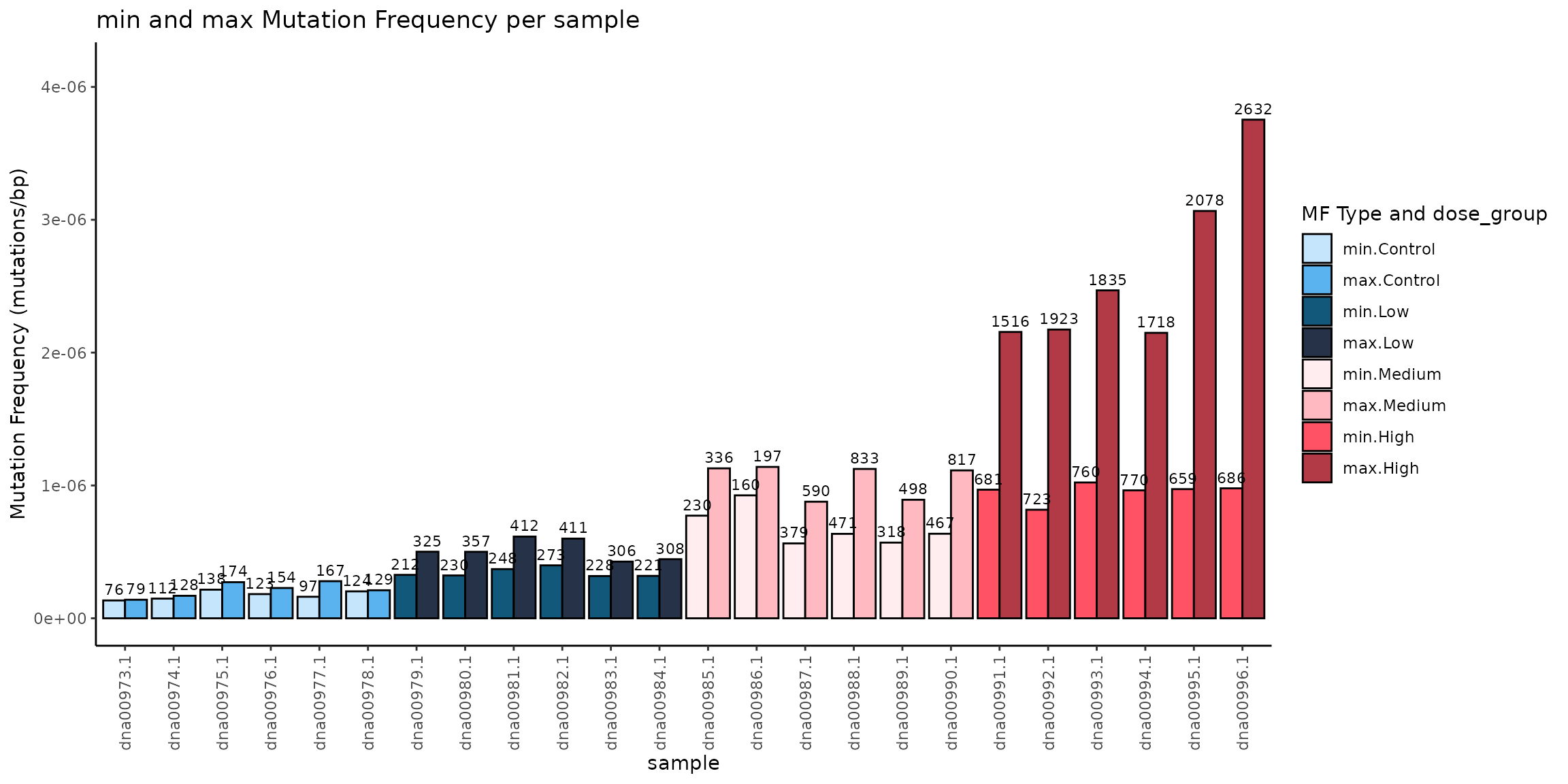

Mutation Frequency (MF) Minimum and Maximum (mutations/bp) per Sample. Light colored bars represent MFmin and dark coloured bars represent MFmax. Bars are coloured and grouped by dose. Data labels are the number of mutations per sample.

plot_mean_mf()

Calculate and plot the mean MF for a user-defined group using plot_mean_mf().

Example 3.11. Plot the mean MF min per dose, including SEM and individual values coloured by dose. See example 3.1 for calculating mf_data_global

plot_mean <- plot_mean_mf(
  mf_data = mf_data_global,
  group_col = "dose_group",
  mf_type = "min",
  fill_col = "dose_group",
  add_labels = "none",
  group_order = "arranged",
  group_order_input = "dose_group",
  plot_legend = FALSE,
  x_lab = "Dose Group"
)
plot_mean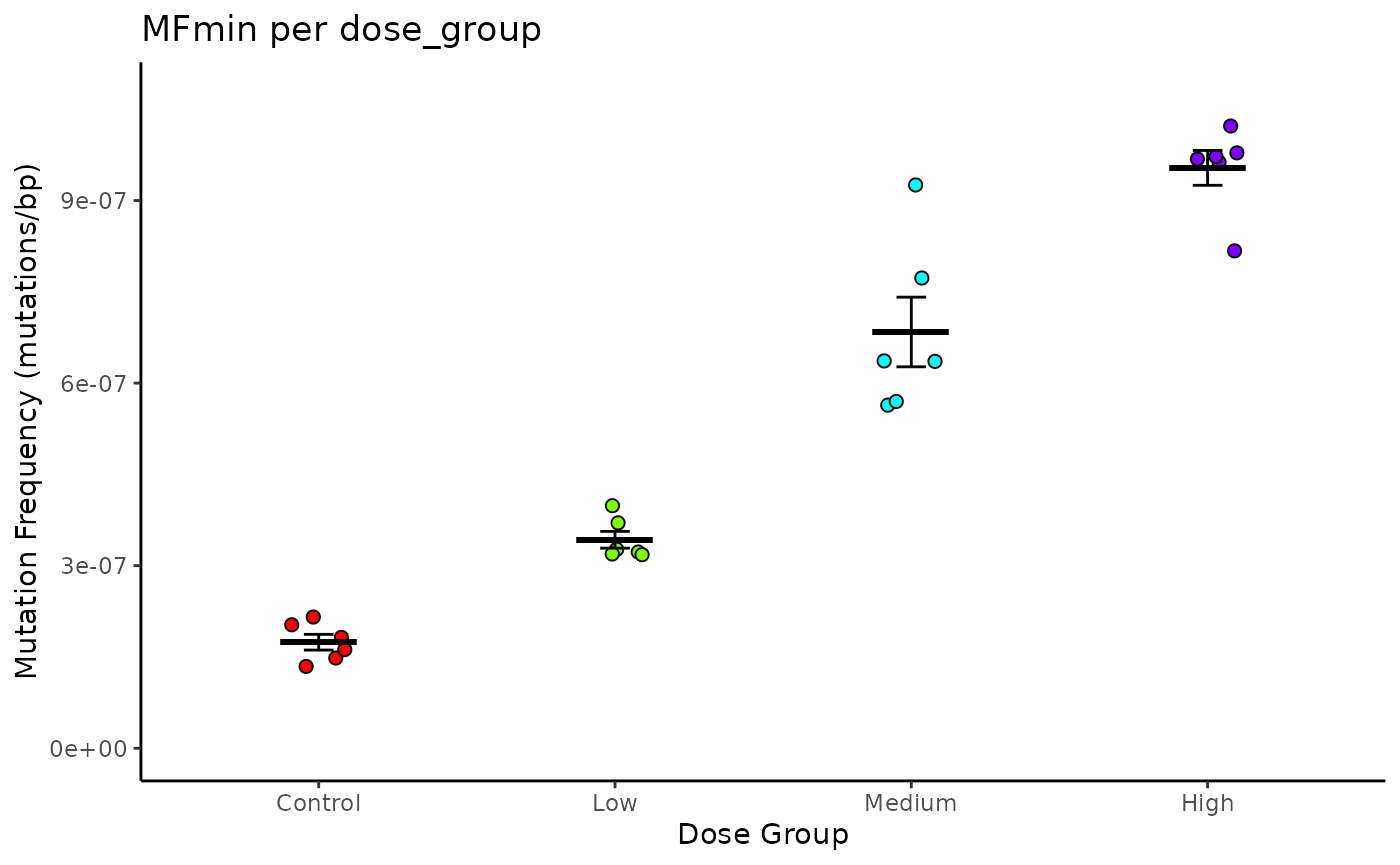

Mean Mutation Frequency (MF) Minimum per Dose. Lines are mean ± S.E.M. Points are individual samples, coloured by dose.

Exporting Results

Users can easily output data frames to an Excel workbook with write_excel(). This function can write single data frames or it can take a list of dataframes and write each one to a separate Excel sheet in a workbook.

In addition to data frames, write_excel() will also extract the mf_data, point_estimates, and pairwise_comparisons from model_mf() output to write to an excel workbook. Set model_results to TRUE if supplying the function with the output to model_mf(). See Modelling Mutation Frequencies for more information on using model_mf().

Example 4.1. Write MF data to excel workbook.

# save a single data frame to an Excel file
write_excel(mf_data_global, workbook_name = "example_mf_data")

# Write multiple data frames to a list to export all at once.
list <- list(mf_data_global, mf_data_rg, mf_data_6)
names(list) <- c("mf_per_sample", "mf_per_region", "mf_6spectra")

#save a list of data frames to an Excel file
write_excel(list, workbook_name = "example_mf_data_list")

Mutation data can be written to a VCF file for downstream applications with write_vcf_from_mut().

Examples 4.2: export our example data as a vcf file.

write_vcf_from_mut(example_data)

Summary Report

To facilitate reproducible analysis of error-corrected sequencing data, the MutSeqR package includes a pre-built R Markdown workflow: Summary_Report.Rmd. This report template allows users to efficiently evaluate the effects of an experimental variable (e.g., dose, age, tissue) on mutation frequency and mutational spectra.

The workflow guides users through a standardized analysis pipeline that includes:

• Mutation data Import
• Mutation data Filtering
• Calculation of Global Mutation Frequencies per Sample
• Visualization of mutation frequencies per Sample and Mean mutation frequencies per experimental group.
• Generalized Linear Modeling of Mutation Frequency (min) as an effect of the experimental variable.
• Optional Benchmark Dose Modeling of mutation frequency across a dose or concentration variable.
• Calculation of Mutation Subtype Frequencies and Proportions at the base-6 and base-96 resolutions.
• Comparison of base-6 mutation spectra between experimental groups.
• Visualization of base-6 subtype proportions per sample with hierarchical clustering
• Visualization of base-6 subtype proportions per experimental group.
• Visualization of base-96 subtype proportions per experimental group.
• Mutation signature analysis per experimental group.
• Generalized Linear Mixed Modeling of mutation frequency as an effect of specified genomic regions and the experimental group.
• Visualization of multiplet mutations per experimental group.

All figures will be included in the report. Data frames included in the report will also be exported to excel workbooks within a predefined output path.

General Usage

Users must download the config file “summary_config.yaml”. This file defines the parameters to be passed to the Summary_Report.rmd. Users must fill out the .yaml file and save it.

config <- system.file("extdata", "inputs", "summary_config.yaml", package = "MutSeqR")
file.copy(from = config, to = "path/to/save/the/summary_config.yaml")

Users can then render the report using MutSeqR’s render_report(). Provide the function with the .yaml file using the config_file_path parameter. Provide the name and the file path of the output file to the output_file parameter. Set the output_format to one of “html_document” (recommended), “pdf_document”, or “all”.

render_report(config_file_path = "path/to/summary_config.yaml",
              output_file = "path/to/output_file.html",
              output_format = "html_document")

Parameters

Below is a description of the parameters set in summary_config.yaml. Parameters are catagerised by their function.

System Set Up

• projectdir: The working directory for the project. All filepaths will be imported from the projectdir. If NULL, the current working directory will be used.
• outputdir: The output directory where output files will be saved. If NULL, the projectdir will be used.

Project Details

• project_title: The project title.
• research_name: The name of the principle investigator for the project.
• user_name: The name of the one running the analysis.
• project_description: Optional description of the project.

Workflow Profile

• config_profile : Choose a workflow profile to load pre-defined parameters. Current options are “Duplex Sequencing Mouse Mutagenesis Panel”, “Duplex Sequencing Human Mutagenesis Panel”, “Duplex Sequencing Rat Mutagenesis Panel”, “CODEC”^1, and “None”. Pre-defined parameters are set to handle data import and filtering. More profiles coming soon. If not using a pre-defined profile (“None”), users must fill out the Custom_Profile_Params (see below).

^1 CODEC .maf files output from the CODECsuite analysis pipeline may be imported provided the user 1. Adds a “sample” column, 2. Adds an “end” column equal to the Start_Position + length(Reference_Allele) - 1, 3. Ensure Chromsome entries are consistent with notation of BSgenome seqnames for the given reference genome. Ex. GRCh38 requires users to remove “chr” from the Chromosome value.

Data Import

• BS_genome: The BS genome to use to populate the sequence context. The given BS genome must be installed prior to running the render_report() function. To identify an appropriate BS genome based on species and genome assembly, use find_BS_genome(). Ex. “BSgenome.Mmusculus.UCSC.mm10”
• file_type: The format of the mutation data to be imported. Options are table or vcf.
• mutation_file: The file path to the mutation data file(s). This can be an individual file or a directory containing multiple files. The file path will be read as projectdir/mutation_file.
• mut_sep: The delimiter for importing tabular mutation data. Ex. “ is tab-delimited.
• sample_data: An optional file path to the sample metadata that will be joined with the mutation data. Set to NULL if not importing metadata. The file path will be read as projectdir/sample_data.
• sd_sep: The delimiter for importing the sample_data file. Ex. “ is tab-delimited.

Calculating MF

Precalculated-depth files: The Summary_Report will automatically check during import whether the mutation data contains a depth column (total_depth or depth). If a depth column does not exist, per-sample precalculated depth can be provided for any subtype resolution to calculate mutation frequencies. If an exp_variable is provided, the Summary_Report will automatically sum the per-sample depths to obtain the depth per experimental group as needed.

In order for MutSeqR to calculate the depth from the mutation data, the data must have the depth-value for every sequenced site. It is not sufficient to calculate the depth from a list of variants. No-variant sites must be included. The Summary Report will check for a total_depth column, but it will not check whether no_variant sites are included. If it finds a total_depth column, it will proceed to calculate the depth from the mutation data.

• precalc_depth_data_global: Optional file path to the precalculated per-sample total_depth data. This is the total number of bases sequenced per sample, used for calculating mutation frequencies. Columns are “sample” and “group_depth”. If using an exp_variable (see below), please also include it in this table. The file path will be read as projectdir/precalc_depth_data_global.
• precalc_depth_data_base6: Optional file path to the precalculated per-sample total_depth data in the base_6 context. This is the total number of C and T bases sequenced for each sample. Columns are “sample”, “normalized_ref”, and “subtype_depth”. If using an exp_variable (see below), please also include it in this table. The file path will be read as projectdir/precalc_depth_data_base6.
• precalc_depth_data_base96: Optional file path to the precalculated per-sample total_depth data in the base_96 context. This is the total number bases sequenced per sample for each of the 32 possible trinucleotide contexts in their pyrimidine notation. Columns are “sample”, “normalized_context”, and “subtype_depth”. If using an exp_variable, please also include it in this table. The file path will be read as projectdir/precalc_depth_data_base96.
• precalc_depth_data_rg: Optional file path to the precalculated per-sample total_depth data for each target region. This is the total number of bases sequenced per sample for each region. Columns are “sample”, ‘region_col’, “group_depth”. Only applicable if performing regions analysis. The file path will be read as projectdir/precalc_depth_data_rg.
• d_sep: The delimiter for importing the precalc_depth_data files.

Statistical Analysis

The Summary Report will run several analyses to investigate the effect of a specified experimental variable on mutation frequency and spectra.

• exp_variable: Optional. The experimental variable of interest. This argument should refer to a column in your mutation data or sample_data. The Summary Report does not support the analysis of multiple exp_variables; supply only one column name. Ex. “dose”. If NULL, statistical analyses will be skipped.
• exp_variable_order: A vector specifying the unique levels of the exp_variable in the order desired for plotting.
• reference_level: The reference level of the exp_variable. Ex. the vehicle control group for a chemical dose. This value must match one of the levels within the exp_variable column. If your experimental variable does not have a reference level, then any level of the variable is fine.
• contrasts: An optional file path to the contrasts table specifying pairwise comparisons between levels of the experimental variable. Required 2 columns, no header. The level in the first column will be compared to the level in the second column for each row. P-values will be adjusted for multiple comparisons if more than one comparison is specified. This contrasts table will be used for Generalized Linear Modeling of MFmin by the exp_variable (model_mf), Generalized Linear Mixed Modeling of MFmin by the exp_variable and target regions, if using a targeted panel (model_mf), and comparing the base_6 mutation spectra between exp_variable levels (spectra_comparison). The file path will be read as projectdir/contrasts. If NULL, spectra_comparison will be skipped, and the GLM/GLMM will return only the model estimates per exp_variable.
• cont_sep: the delimiter for importing the contrasts file.
• bmd: A logical variable indicating whether to run a BMD analysis on the MF data. If TRUE, the exp_variable must refer to numeric dose or concentration values.
• bmr: A numeric value indicating the benchmark response for the bmd analysis. The Summary Report defines the bmr as a bmr-% increase in MF from the reference level. Default is 0.5.

Custom Profile Parameters

Users who do not wish to use one of the pre-defined parameter profiles may still run the Summary Report by filling out the Custom_Profile_Params. If using one of the config_profiles, users should skip this section.

• ecs_technology: The technology used to generate the data.
• is_0_based_mut: A logical variable indicating whether the genomic coordinates of the tabular mutation data are 0-based (TRUE), or 1-based (FALSE).
• regions: An optional file path to the regions metadata file. The file must contain columns “contig”, “start”, “end” in addition to the metadata.
• is_0_based_rg: A logical variable indicating whether the genomic coordinates of the regions file are 0-based (TRUE), or 1-based (FALSE).
• rg_sep: The delimiter for importing the regions file.
• vaf_cutoff: A numeric value from 0-1. Will flag variants with a VAF > vaf_cutoff as germline variants and filter them from mutation counts.
• snv_in_germ_mnv: A logical variable indicating whether filter_mut should flag SNVs that overlap with germline MNVs for filtering.
• rm_abnormal_vaf: A logical variable indicaring whether filter_mut should remove records where the VAF is between 0.05-0.45 or between 0.55-0.95.
• custom_filter_col: A column name used by filter_mut to apply a custom filter to the specified column.
• custom_filter_val: The value in custom_filter_col by which to filter.
• custom_filter_rm: A logical variable indicating whether records that contain the custom_filter_val within the custom_filter_col should be removed (TRUE) or flagged (FALSE).
• filtering_regions: Optional file path to regions file by which to filter variants. Must contain the contig, start, and end of each region. The file path will be read as projectdir/filtering_regions.
• filtering_rg_sep: The delimiter for importing the filtering_regions file.
• regions_filter: “keep_within” will remove any records that fall outside of the filtering_regions. “remove_within” will remove records that fall inside of the filtering_regions.
• allow_half_overlap: A logical variable indicating whether to include records that half overlap with the regions. If FALSE, the start and end position of the record must fall within the region interval to be counted as “falling in the region”. If TRUE, records that start/end within the region interval, but extend outside of it will be counted as “falling inside the region”.
• filtering_is_0_based_rg: A logical variable indicating whether the genomic coordinates of the filtering_regions are 0-based (TRUE) or 1-based (FALSE).
• rm_filtered_mut_from_depth: A logical variable indicating whether the alt_depth of variants flagged during the filtering process should be removed from their total_depth values. This does not apply to records flagged as germline variants.
• do_regions_analysis: A logical variable indicating whether to perform Generalized Linear Mixed Modeling of the data by sequencing target. This is applicable to data sets that used a targeted panel or has specific regions of interest.
• region_col: The column name that uniquely identifies each target region for the regions_analysis. This column must be present in the mutation_data or in the regions metadata file.

Output

render_report() will output the summary report of results as an html file or a pdf file. All output will be saved to the output_directory specified in the summary_config.yaml.

Report

The Summary Report consists of the following sections.

1. Import the Mutation Data: Statement of number of imported rows and the total number of samples detected.
2. Filter the Mutation Data: Summary of applied filters with total counts for the number of records that were flagged/removed.
3. Calculate Per-Sample Mutation Frequency: Mutation frequency calculated per sample. Includes plot of mutation frequency per sample and plot of mean mutation frequency per experimental group (given experimental variable was provided).
4. Generalized Linear Modelling: Model results of mutation frequency as an effect of the experimental variable. Includes model summary, residual plots, model estimates, pairwise comparisons as specified in “contrasts”, and a plot of the model estimates and significant results.
5. Benchmark Dose Analysis: BMD results for the experimental variable on mutation frequency. BMD estimates per individual model and model-averaged result. Includes model plots, cleveland plots, and confidence interval plots.
6. 6-Base Spectrum: Mutation frequency calculated at the base_6 resolution per-sample and averaged across the experimental variable. Includes hierarchical clustering of samples by subtype proportion, spectra comparison between experimental groups, and plot of subtype proportions per experimental group.
7. 96-Base Trinucleotide Spectrum: Mutation frequency calculated at the base_96 resolution per-sample and averaged across the experimental variable. Includes trinucleotide proportion plots for all experimental groups or by sample if no experimental variable is provided.
8. Regions Analysis: Mutation frequency calculated per sample for genomic regions of interest. Includes model results of mutation frequency as an effect of the experimental variable and genomic target. Pairwise comparisons specified in contrasts are conducted for each genomic target individually. If no experimental variable is provided, model results reflect mutation frequency as an effect of genomic target.
9. Mutation HotSpots: Statement # of mutations that occur in more than one sample. Also includes recurrent mutations within experimental groups.
10. Lollipop Plots: Given genomic regions of interest, plots recurrent mutations across genomic position.
11. Bubble Plot: Multiple Mutations: Bubble plot depicting multiplet mutations per experimental group.

If an experimental variable is not provided, statistical analysis will be skipped.

References

Appendix

Session Info

## R Under development (unstable) (2025-11-18 r89035)
## Platform: x86_64-pc-linux-gnu
## Running under: Ubuntu 24.04.3 LTS
## 
## Matrix products: default
## BLAS:   /usr/lib/x86_64-linux-gnu/openblas-pthread/libblas.so.3 
## LAPACK: /usr/lib/x86_64-linux-gnu/openblas-pthread/libopenblasp-r0.3.26.so;  LAPACK version 3.12.0
## 
## locale:
##  [1] LC_CTYPE=C.UTF-8       LC_NUMERIC=C           LC_TIME=C.UTF-8       
##  [4] LC_COLLATE=C.UTF-8     LC_MONETARY=C.UTF-8    LC_MESSAGES=C.UTF-8   
##  [7] LC_PAPER=C.UTF-8       LC_NAME=C              LC_ADDRESS=C          
## [10] LC_TELEPHONE=C         LC_MEASUREMENT=C.UTF-8 LC_IDENTIFICATION=C   
## 
## time zone: UTC
## tzcode source: system (glibc)
## 
## attached base packages:
## [1] stats4    stats     graphics  grDevices utils     datasets  methods  
## [8] base     
## 
## other attached packages:
##  [1] BSgenome.Mmusculus.UCSC.mm10_1.4.3 BSgenome_1.79.1                   
##  [3] rtracklayer_1.71.0                 BiocIO_1.21.0                     
##  [5] Biostrings_2.79.2                  XVector_0.51.0                    
##  [7] GenomicRanges_1.63.0               Seqinfo_1.1.0                     
##  [9] IRanges_2.45.0                     S4Vectors_0.49.0                  
## [11] ExperimentHub_3.1.0                AnnotationHub_4.1.0               
## [13] BiocFileCache_3.1.0                dbplyr_2.5.1                      
## [15] BiocGenerics_0.57.0                generics_0.1.4                    
## [17] MutSeqR_0.99.3                     htmltools_0.5.8.1                 
## [19] DT_0.34.0                         
## 
## loaded via a namespace (and not attached):
##  [1] DBI_1.2.3                   bitops_1.0-9               
##  [3] httr2_1.2.1                 rlang_1.1.6                
##  [5] magrittr_2.0.4              matrixStats_1.5.0          
##  [7] compiler_4.6.0              RSQLite_2.4.4              
##  [9] GenomicFeatures_1.63.1      png_0.1-8                  
## [11] systemfonts_1.3.1           vctrs_0.6.5                
## [13] stringr_1.6.0               pkgconfig_2.0.3            
## [15] crayon_1.5.3                fastmap_1.2.0              
## [17] labeling_0.4.3              Rsamtools_2.27.0           
## [19] rmarkdown_2.30              ragg_1.5.0                 
## [21] purrr_1.2.0                 bit_4.6.0                  
## [23] xfun_0.54                   cachem_1.1.0               
## [25] cigarillo_1.1.0             jsonlite_2.0.0             
## [27] blob_1.2.4                  DelayedArray_0.37.0        
## [29] BiocParallel_1.45.0         parallel_4.6.0             
## [31] R6_2.6.1                    plyranges_1.31.1           
## [33] VariantAnnotation_1.57.0    bslib_0.9.0                
## [35] stringi_1.8.7               RColorBrewer_1.1-3         
## [37] jquerylib_0.1.4             SummarizedExperiment_1.41.0
## [39] knitr_1.50                  Matrix_1.7-4               
## [41] tidyselect_1.2.1            dichromat_2.0-0.1          
## [43] abind_1.4-8                 yaml_2.3.10                
## [45] codetools_0.2-20            curl_7.0.0                 
## [47] lattice_0.22-7              tibble_3.3.0               
## [49] Biobase_2.71.0              withr_3.0.2                
## [51] KEGGREST_1.51.1             S7_0.2.1                   
## [53] evaluate_1.0.5              desc_1.4.3                 
## [55] pillar_1.11.1               BiocManager_1.30.27        
## [57] filelock_1.0.3              MatrixGenerics_1.23.0      
## [59] rprojroot_2.1.1             RCurl_1.98-1.17            
## [61] BiocVersion_3.23.1          ggplot2_4.0.1              
## [63] scales_1.4.0                glue_1.8.0                 
## [65] tools_4.6.0                 data.table_1.17.8          
## [67] GenomicAlignments_1.47.0    fs_1.6.6                   
## [69] XML_3.99-0.20               grid_4.6.0                 
## [71] tidyr_1.3.1                 crosstalk_1.2.2            
## [73] colorspace_2.1-2            AnnotationDbi_1.73.0       
## [75] restfulr_0.0.16             cli_3.6.5                  
## [77] rappdirs_0.3.3              textshaping_1.0.4          
## [79] S4Arrays_1.11.0             ggdendro_0.2.0             
## [81] dplyr_1.1.4                 gtable_0.3.6               
## [83] sass_0.4.10                 digest_0.6.39              
## [85] SparseArray_1.11.2          rjson_0.2.23               
## [87] htmlwidgets_1.6.4           farver_2.1.2               
## [89] memoise_2.0.1               pkgdown_2.2.0              
## [91] lifecycle_1.0.4             httr_1.4.7                 
## [93] here_1.0.2                  bit64_4.6.0-1              
## [95] MASS_7.3-65

Danecek, Petr, Adam Auton, Goncalo Abecasis, Cornelis A. Albers, Eric Banks, Mark A. DePristo, Robert E. Handsaker, et al. 2011. “The Variant Call Format and VCFtools.” Bioinformatics 27 (15): 2156–58. https://doi.org/10.1093/bioinformatics/btr330.

Dodge, Annette E., Danielle P. M. LeBlanc, Gu Zhou, Andrew Williams, Matthew J. Meier, Phu Van, Fang Yin Lo, et al. 2023. “Duplex Sequencing Provides Detailed Characterization of Mutation Frequencies and Spectra in the Bone Marrow of MutaMouse Males Exposed to Procarbazine Hydrochloride.” Archives of Toxicology 97 (8): 2245–59. https://doi.org/10.1007/s00204-023-03527-y.

Kennedy, Scott R., Michael W. Schmitt, Edward J. Fox, Brendan F. Kohrn, Jesse J. Salk, Eun Hyun Ahn, Marc J. Prindle, et al. 2014. “Detecting Ultralow-Frequency Mutations by Duplex Sequencing.” Nature Protocols 9 (11): 2586–606. https://doi.org/10.1038/nprot.2014.170.

LeBlanc, Danielle P. M., Matthew Meier, Fang Yin Lo, Elizabeth Schmidt, Charles Valentine, Andrew Williams, Jesse J. Salk, Carole L. Yauk, and Francesco Marchetti. 2022. “Duplex Sequencing Identifies Genomic Features That Determine Susceptibility to Benzo(a)pyrene-Induced in Vivo Mutations.” BMC Genomics 23 (1): 542. https://doi.org/10.1186/s12864-022-08752-w.

Marchetti, Francesco, Renato Cardoso, Connie L. Chen, George R. Douglas, Joanne Elloway, Patricia A. Escobar, Tod Harper Jr, et al. 2023. “Error-Corrected Next-Generation Sequencing to Advance Nonclinical Genotoxicity and Carcinogenicity Testing.” Nature Reviews Drug Discovery 22 (3): 165–66. https://doi.org/10.1038/d41573-023-00014-y.

Marchetti, Francesco, Renato Cardoso, Connie L. Chen, George R. Douglas, Joanne Elloway, Patricia A. Escobar, Tod Harper, et al. 2023. “Error-Corrected Next Generation Sequencing - Promises and Challenges for Genotoxicity and Cancer Risk Assessment.” Mutation Research. Reviews in Mutation Research 792: 108466. https://doi.org/10.1016/j.mrrev.2023.108466.

Menon, Vijay, and Douglas E. Brash. 2023. “Next-Generation Sequencing Methodologies to Detect Low-Frequency Mutations: ‘Catch Me If You Can’.” Mutation Research/Reviews in Mutation Research 792 (July): 108471. https://doi.org/10.1016/j.mrrev.2023.108471.