Perform linear modelling on mutation frequency for given fixed and random effects

model_mf will fit a linear model to analyse the effect(s) of given factor(s) on mutation frequency and perform specified pairwise comparisons. This function will fit either a generalized linear model (glm) or, if supplied random effects, a generalized linear mixed-effects model (glmer). Pairwise comparisons are conducted using the doBy library (esticon) and estimates are then back-transformed. The delta method is employed to approximate the back-transformed standard-errors. A Sidak correction is applied to adjust p-values for multiple comparisons.

Usage

model_mf(
  mf_data,
  fixed_effects,
  test_interaction = TRUE,
  random_effects = NULL,
  reference_level,
  muts = "sum_min",
  total_count = "group_depth",
  contrasts = NULL,
  cont_sep = "\t",
  ...
)

Arguments

mf_data: The data frame containing the mutation frequency data. Mutation counts and total sequencing depth should be summarized per sample alongside columns for your fixed effects. This data can be obtained using calculate_mf(summary=TRUE).
fixed_effects: The name(s) of the column(s) that will act as the fixed_effects (factor/independent variable) for modelling mutation frequency.
test_interaction: a logical value. Whether or not your model should include the interaction between the fixed_effects.
random_effects: The name of the column(s) to be analysed as a random effect in the model. Providing this effect will cause the function to fit a generalized linear mixed-effects model.
reference_level: Refers to one of the levels within each of your fixed_effects. The coefficient for the reference level will represent the baseline effect. The coefficients of the other levels will be interpreted in relation to the reference_level as deviations from the baseline effect.
muts: The column containing the mutation count per sample.
total_count: The column containing the sequencing depth per sample.
contrasts: a data frame or a filepath to a file that will provide the information necessary to make pairwise comparisons between groups. The table must consist of two columns. The first column will be a group within your fixed_effects and the second column must be the group that it will be compared to. The values must correspond to entries in your mf_data column for each fixed effect. Put the group that you expect to have the higher mutation frequency in the 1st column and the group that you expect to have a lower mutation frequency in the second column. For multiple fixed effects, separate the levels of each fixed_effect of a group with a colon. Ensure that all fixed_effects are represented in each entry for the table. See details for examples.
cont_sep: The delimiter for importing the contrast table file. Default is tab-delimited.
...: Extra arguments for glm or glmer. The glmer function is used when a random_effect is supplied, otherwise, the model uses the glm function.

Value

Model results are output as a list. Included are:

model_data: the supplied mf_data with added column for the Pearson's residuals of the model.
summary: the summary of the model.
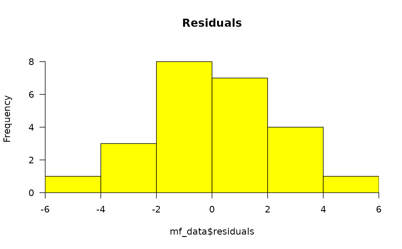
anova: the analysis of variance for models with two or more effects. Anova(model)
residuals_histogram: the Pearson's residuals plotted as a histogram. This is used to check whether the variance is normally distributed. A symmetric bell-shaped histogram, evenly distributed around zero indicates that the normality assumption is likely to be true.
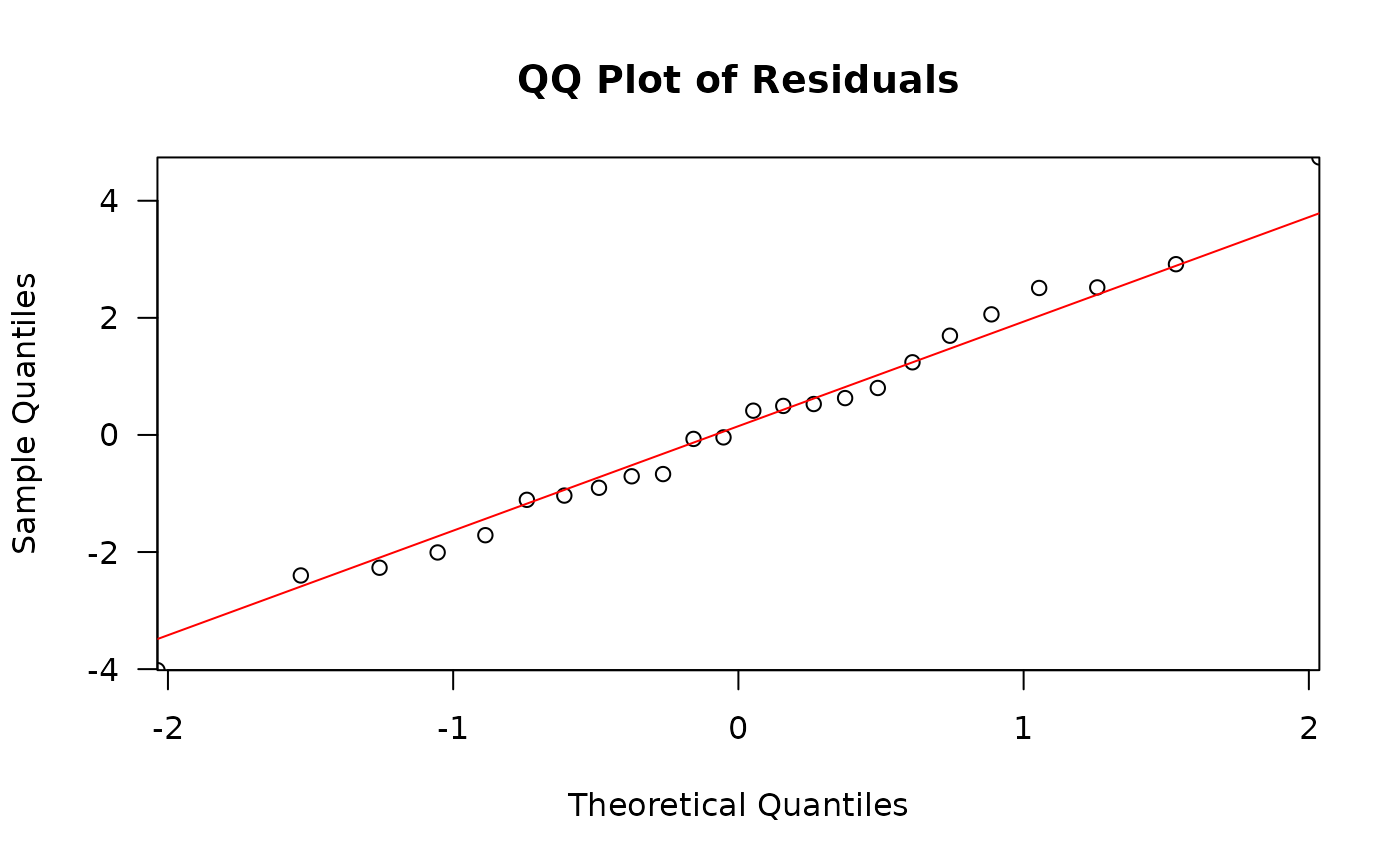
residuals_qq_plot: the Pearson's residuals plotted in a quantile-quantile plot. For a normal distribution, we expect points to roughly follow the y=x line.
point_estimates_matrix: the contrast matrix used to generate point-estimates for the fixed effects.
point_estimates: the point estimates for the fixed effects.
pairwise_comparisons_matrix: the contrast matrix used to conduct the pairwise comparisons specified in the contrasts.
pairwise_comparisons: the results of pairwise comparisons specified in the contrasts.

Details

fixed_effects are variables that have a direct and constant effect on the dependent variable (ie mutation frequency).They are typically the experimental factors or covariates of interest for their impact on the dependent variable. One or more fixed_effect may be provided. If you are providing more than one fixed effect, avoid using correlated variables; each fixed effect must independently predict the dependent variable. Ex. fixed_effects = c("dose", "genomic_target", "tissue", "age", etc).

Interaction terms enable you to examine whether the relationship between the dependent and independent variable changes based on the value of another independent variable. In other words, if an interaction is significant, then the relationship between the fixed effects is not constant across all levels of each variable. Ex. Consider investigating the effect of dose group and tissue on mutation frequency. An interaction between dose and tissue would capture whether the dose response differs between tissues.

random_effects account for the unmeasured sources of statistical variance that affect certain groups in the data. They help account for unobserved heterogeneity or correlation within groups. Ex. If your model uses repeated measures within a sample, random_effects = "sample".

Setting a reference_level for your fixed effects enhances the interpretability of the model. Ex. Consider a fixed_effect "dose" with levels 0, 25, 50, and 100 mg/kg. Intuitively, the reference_level would refer to the negative control dose, "0" since we are interested in testing how the treatment might change mutation frequency relative to the control.

Examples of contrasts:

If you have a fixed_effect "dose" with dose groups 0, 25, 50, 100, then the first column would contain the treated groups (25, 50, 100), while the second column would be 0, thus comparing each treated group to the control group.

25 0

50 0

100 0

Alternatively, if you would like to compare mutation frequency between treated dose groups, then the contrast table would look as follows, with the lower dose always in the second column, as we expect it to have a lower mutation frequency. Keeping this format aids in interpretability of the estimates for the pairwise comparisons. Should the columns be reversed, with the higher group in the second column, then the model will compute the fold-decrease instead of the fold-increase.

100 25

100 50

50 25

Ex. Consider the scenario where the fixed_effects are "dose" (0, 25, 50, 100) and "genomic_target" ("chr1", "chr2"). To compare the three treated dose groups to the control for each genomic target, the contrast table would look like:

25:chr1 0:chr1

50:chr1 0:chr1

100:chr1 0:chr1

25:chr2 0:chr2

50:chr2 0:chr2

100:chr2 0:chr2

Troubleshooting: If you are having issues with convergence for your generalized linear mixed- effects model, it may be advisable to increase the tolerance level for convergence checking during model fitting. This is done through the control argument for the lme4::glmer function. The default tolerance is tol = 0.002. Add this argument as an extra argument in the model_mf function. Ex. control = lme4::glmerControl(check.conv.grad = lme4::.makeCC("warning", tol = 3e-3, relTol = NULL))

Examples

# Example data consists of 24 mouse bone marrow DNA samples imported
# using import_mut_data() and filtered with filter_mut.
# Data was summarized per sample using calculate_mf() (see relevant
# examples). We will run the model with model_mf then plot the results.
mf_example <- readRDS(system.file("extdata/Example_files/mf_data_global.rds",
  package = "MutSeqR"
))
# We will compare all treated groups to the control group
contrasts <- data.frame(
  col1 = c("12.5", "25", "50"),
  col2 = c("0", "0", "0")
)
# Fit the model
model <- model_mf(
  mf_data = mf_example,
  fixed_effects = "dose",
  reference_level = "0",
  muts = "sum_min",
  total_count = "group_depth",
  contrasts = contrasts
)
#> Reference level for factordose:0
#> Fitting generalized linear model. glm(cbind( sum_min , group_depth ) ~  dose, family = quasibinomial
#> The highest residual in absolute value is:4.73969242941171in row:14



# Plot the results using plot_model_mf()
plot <- plot_model_mf(model,
  plot_type = "bar",
  x_effect = "dose",
  plot_error_bars = TRUE,
  plot_signif = TRUE,
  x_order = c("0", "12.5", "25", "50"),
  x_label = "Dose (mg/kg-bw/d)",
  y_label = "Estimated Mean MF (mutations/bp)",
  plot_title = ""
)
#> Joining with `by = join_by(dose)`