Create a radar plot
Examples
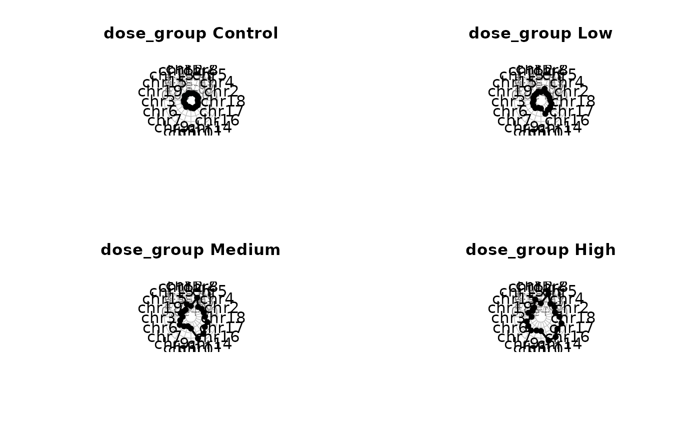
# Plot the MFmin for each variation type, including the 6 SNV subtypes
# Facet the plots by dose group
mf_ex <- readRDS(system.file("extdata", "Example_files", "mf_data_6.rds",
     package = "MutSeqR")
)
plot <- plot_radar(
     mf_data = mf_ex,
     response_col = "mf_min",
     label_col = "normalized_subtype",
     facet_col = "dose_group",
     indiv_y = TRUE
)